Вывод сечения

Доступны два типа вывода сечения.

Первый — это вывод истории времени /TH/SECTIO, состоящий из суммы силы и моментов, действующих на сечение. Вывод может быть в глобальной системе или локальной системе, при этом наиболее распространенным выводом являются группы переменных, GLOBAL, LOCAL и CENTER.

Второй тип вывода — это смещения и необязательные сила и момент для каждого узла в сечении, записанные в файл выходных данных сечения SC01. Затем этот файл можно прочитать как наложенное смещение, примененное ко второй модели сечения разреза. Методология RD-E: 5400 Cut — это пример методологии сечения разреза, которую можно использовать. В этом случае полная модель запускается с I_SAVE =1 или 2 для сохранения перемещения и, при необходимости, результирующих сил/моментов сечения в файле file_nameSC01.

Затем создается вторая модель разреза (подмодель) с разделом, определенным с помощью опции I_SAVE =100 или 101 для чтения смещения узлов файла раздела. Локальная система раздела, определяемая тремя узлами node_ID₁, node_ID₂ и node_ID₃ или frame_ID, должна быть той же, которая использовалась при сохранении данных (I_SAVE =1 или 2) и чтении данных (I_SAVE =100 или 101).

Если I_SAVE =2 используется в полной модели, а I_SAVE =101 используется в модели разреза, то PRADIOS выводит разницу между результирующими силами и моментами сечения в полной и разрезной модели в сечении (/TH/ SECTIO).

Для улучшения времени решения и уменьшения необходимой памяти рекомендуется установить I_SAVE =0, если методология моделирования разреза не требуется.

Фильтр

При считывании и применении смещений к модели сечения разреза, смещение можно отфильтровать с помощью фильтра экспоненциального скользящего среднего. Например, отфильтрованное смещение в направлении x будет:

\[x_{f}=\alpha x(t)+(1-\alpha)x(t-dt) \tag{49}\]

Где,

\(x_{f}\) Фильтрованное смещение

\(\alpha\) Константа фильтрации экспоненциального скользящего среднего

\(x(t)\) Неотфильтрованное смещение в текущий момент времени

\(x(t-dt)\) Смещение на предыдущем временном шаге

Рекомендации:

\(\alpha =\frac{2\pi dt}{T}\) для фильтрации -3 дБ

\(\alpha =\frac{2\pi dt}{\sqrt{3T}}\) для фильтрации -6 дБ

Где,

\(T\) Период фильтрации

\(dt\) Шаг времени модели

Период фильтрации \(T = 10\Delta t\) часто используется, что делает \(\alpha =\frac{2\pi}{10}\) = 0,62832 для фильтра -3 дБ.

Материалы

Различные испытания материалов могут привести к различным механическим характерам материала.

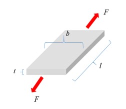
Типичным испытанием материала для металла является испытание на растяжение. С помощью этого испытания можно наблюдать кривую напряжения и деформации, предел текучести, точку сужения и точку разрушения материала.

width

2.10018in

height

1.80849in

Рисунок 131: Измеряются сила (F) и длина (l)

Инженерная кривая деформации-напряжения может быть сгенерирована следующим образом:

\[\sigma_{e}=\frac{F}{S_{0}} \tag{50}\]

\[c_{e}=\frac{\Delta I}{I_{0}} \tag{51}\]

Где,

\(S_{0}\) Площадь сечения в исходном состоянии

\(I_{0}\) Начальная длина

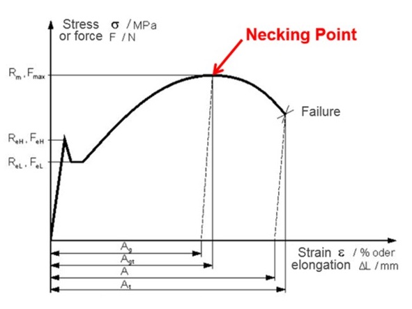
В этой кривой сила-удлинение или инженерной кривой напряжение-деформация важны три точки.

1. Предел текучести: где материал начинает течь. До текучести можно предположить, что материал находится в упругом состоянии (можно измерить модуль Юнга E), а после текучести — пластическая деформация материала, которая необратима.

• Некоторые материалы в этом тесте сначала достигнут верхнего предела текучести (R_eH), а затем упадут до нижнего предела текучести (R_eL). На инженерной кривой напряжения-деформации можно взять нижний предел текучести (консервативное значение).

• Некоторые материалы не могут легко найти предел текучести. Возьмите напряжение 0,1 или 0,2% пластической деформации в качестве предела текучести.

2. Точка сужения: где материал достигает максимального напряжения на инженерной кривой напряжения-деформации. После этой точки материал начинает размягчаться.

3. Точка разрушения: где материал разрушился.

width

5.15045in

height

3.83367in

Рисунок 132:

\(\mathbf{R_{m}}\) Максимальное сопротивление

\(\mathbf{F_{max}}\) Максимальная сила

\(\mathbf{R_{eH}}\) Верхний предел текучести

\(\mathbf{R_{eL}}\) Нижний предел текучести

\(\mathbf{A_{g}}\) Равномерное удлинение

\(\mathbf{A_{gt}}\) Общее равномерное удлинение

\(\mathbf{A_{t}}\) Полная деформация разрушения

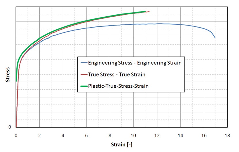
Истинная кривая напряжения-деформации, которая требуется для большинства материалов в PRADIOS, за исключением LAW2, где как инженерное напряжение-деформация, так и истинное напряжение-деформация возможны для ввода данных о материалах.

На рисунке 133 найдите инженерную кривую напряжения-деформации (синюю) с помощью:

\[\sigma_{tr}=\sigma_{e}\text{exp}\Big{(}\varepsilon_{tr}\Big{)} \tag{52}\]

\[\varepsilon_{tr}=\text{ln}\big{(}1+\varepsilon_{e}\big{)} \tag{53}\]

Результатом является истинная кривая напряжения-деформации (красная). Пластическая истинная кривая напряжения-деформации показана зеленым цветом, где пластическая деформация начинается с 0. Эта зеленая кривая пластического истинного напряжения-деформации - то, что вам нужно, как в LAW36, LAW60, LAW63 и так далее.

width

6.93393in

height

4.40872in

Рисунок 133:

Истинная кривая напряжения-деформации действительна до точки сужения материала. После точки сужения кривая материала должна быть определена вручную для закалки. Используя другой закон материала, PRADIOS экстраполирует истинную кривую напряжения-деформации до 100%.

• Линейная экстраполяция: если кривая напряжения-деформации является входной функцией (LAW36), то кривая напряжения-деформации линейно экстраполируется с наклоном, определяемым двумя последними точками кривой. Рекомендуется, чтобы список значений абсциссы был увеличен до значения, большего, чем предыдущее значение абсциссы.

• Джонсон-Кук: после точки шейки упрочнение Джонсона-Кука является одним из наиболее часто используемых для экстраполяции истинной кривой напряжения-деформации.

\[\sigma_{y}=a+b\varepsilon_{pn}\]

Однако это может переоценить деформационное упрочнение для автомобильной стали. В этом случае комбинация упрочнения Свифта-Воуса будет более точной.

• Swift и Voce: после точки шейки используйте одно из следующих уравнений для экстраполяции истинной кривой напряжения-деформации.

  Модель Swift

  \(\sigma_{y}=A\left(\varepsilon_{p}+\varepsilon_{0}\right)^{n}\)

  \(A\text{ и } n \text{ положительны.}\)

  Модель Voce

  \(\sigma_{y}=k_{0}+Q\left[1-\exp\left(-B\varepsilon_{p}\right)\right]\)

  \(k_{0,}Q и B\) положительны

Combination of Switch and

Voce model (LAW84 and LAW87)

\(\sigma_{y}=\alpha\big{[}A\big{(}\overline{\varepsilon}_{p}+\varepsilon_{0}\big{)}^{n}\big{]}+(1-\alpha)\big{\{}{k_{0}+Q\big{[}1-exp\big{(}-B\overline{\varepsilon}\{p}\big{)}\big{]}\big{\}}\)

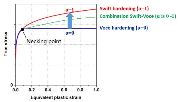
Figure 134:

Здесь α — вес упрочнения Swift и упрочнения Voce. Вот один Скрипт Compose в качестве примера для подгонки параметров упрочнения Swift \(A,\varepsilon_{0}, n\) и параметров упрочнения Voce \(k_{0,} Q, B\) с входной кривой напряжения-деформации.

См. также

/MAT/LAW84 (Starter)

/MAT/LAW87 (BARLAT2000) (Starter)

Гиперупругие материалы

Гиперупругие материалы используются для моделирования материалов, которые реагируют упруго при очень больших деформациях. Эти материалы обычно показывают нелинейную упругую, несжимаемую реакцию деформации напряжения, которая возвращается в исходное состояние при разгрузке.

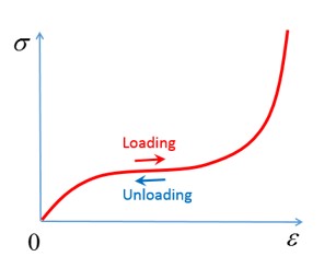
Рисунок 135:

Гиперупругие материалы являются частным случаем материала Коши, где напряжение зависит только от текущей деформации. Кинетическая теория Мейера описывает, как эти материалы состоят из гибкой цепочечной структуры, которая вращается и выпрямляется при деформации. Это привело к теории, согласно которой функция плотности энергии деформации может быть записана как функция деформации.³ Плотность энергии деформации затем может быть дифференцирована для получения поведения напряжения-деформации материала. Наиболее распространенными гиперэластичными материалами являются эластомеры или резины. Некоторые свойства эластомеров включают.²

• Материал почти идеально эластичен, а деформация обратима, причем напряжение является функцией только текущей деформации и не зависит от истории или скорости нагрузки, если деформируется при постоянной температуре или адиабатически.

• Материал несжимаем и сильно сопротивляется изменениям объема. Модуль объемной упругости, который является отношением изменения объема к гидростатическому компоненту напряжения, сопоставим с модулем металлов.

• Материал очень слаб при сдвиге, его модуль сдвига в 10^-5 раз меньше, чем у большинства металлов.

• Материал изотропен, его реакция напряжения-деформации не зависит от ориентации материала.

Рекомендации по свойствам элемента

При использовании гиперупругих материальных законов есть некоторые рекомендуемые настройки свойств элементов. При использовании твердых элементов всегда лучше создавать сетку с 8-узловыми элементами /BRICK, если это возможно. Если нет, то можно использовать элементы /TETRA4 или /TETRA10. Рекомендуемые /PROP/SOLID для 8-узлового кирпича: \(I_{smstr}\) =10, \(I_{cpre}\) =1, с \(I_{solid}\) =24. Если возникает эффект песочных часов, то можно использовать \(I_{solid}\) =17 с \(I_{frame}\) =2.

3. Treloar, L. R. G. “The elastic and related properties of rubbers”. Reports on progress in physics 36, no. 7 (1973): 755

4. Боуэр, Аллан Ф. Прикладная механика твердых тел. CRC press, 2009

Ogden Materials

Гиперупругие материалы можно использовать для моделирования изотропного, нелинейного упругого поведения резины, полимеров и подобных материалов. Эти материалы практически несжимаемы в своем поведении и могут быть растянуты до очень больших деформаций.

В PRADIOS материальные законы LAW42, LAW62, LAW69, LAW82 и LAW88 используют различные функции плотности энергии деформации модели материалов Огдена⁵ для моделирования гиперупругих материалов.⁶

Определение материала

Растяжение (также называемое коэффициентом растяжения) \(\lambda\) — это отношение конечной длины и начальной длины. Используется для материалов с большими деформациями. Для куба при растяжении:

\(\varepsilon_{1}=\frac{\Delta I}{I_{01}}\) Техническая деформация (также называемая номинальной деформацией) в направлении 1

\(\lambda_{1}=\frac{I_{1}}{I_{01}}\) Прочность в направлении 1

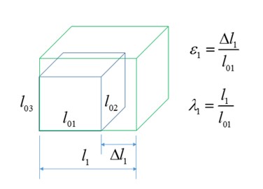
Рисунок 136:

Таким образом, деформация и растяжение связаны следующим образом:

\[\lambda= 1 + \varepsilon \tag{113}\]

Основное растяжение \(\lambda_{i}\) можно использовать для описания объемной деформации путем расчета относительного объема J, вычисляемого как:

\[J=\frac{V}{V_{0}}=\frac{I_{1}\cdot I_{2}\cdot I_{3}}{I_{01}\cdot I_{02}\cdot I _{03}}=\lambda_{1}\cdot\lambda_{2}\cdot\lambda_{3} \tag{114}\]

Для несжимаемого материала объем не должен меняться и, таким образом, =1 и, таким образом, растяжение можно рассчитать для следующих испытаний материалов.

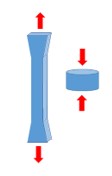
• Одноосный тест:

\(\lambda_{1}=\lambda\text{ и }\lambda_{2}=\lambda_{3}2=\frac{1}{\lambda}\)

• Двуосный тест:

\(\lambda_{1}=\lambda_{2}=\lambda и (\lambda_{3}=\lambda^{-2})\)

• Плоскостной (сдвиговой) тест:

\(\lambda_{1}=\lambda; \lambda_{3}=1 и (\lambda_{2}=\lambda^{-1})\)

/MAT/LAW42 (Ogden)

Эта модель материала определяет гиперупругий, вязкий и несжимаемый материал, заданный с использованием моделей материалов Огдена, Нео-Хука или Муни-Ривлина. Этот закон обычно используется для моделирования несжимаемых резин, полимеров, пен и эластомеров. Этот материал может использоваться с оболочечными и твердыми элементами.

LAW42 использует следующее представление плотности энергии деформации материальной модели Огдена.

\[W\big{(}\lambda_{1},\lambda_{2},\lambda_{3}\big{)}=\sum_{p=1}^{5}\frac{u_{p}}{\alpha_{p}}\big{(}\vec{\lambda}_{1}\alpha_{p}+\vec{\lambda}_{2}\alpha_{p}+\vec{\lambda}_{3}\alpha_{p}-3\big{)}+\frac{K}{2}\big{(}J-1\big{)}^{2}\]

Где,

\(W\) Плотность энергии деформации

\(\lambda_{1}\) \(i_{th}\) главный инженерный участок

\(J\) Относительный объем определяется как: \(J=\lambda_{1}\cdot\lambda_{2}\cdot\lambda_{3}=\frac{\rho_{0}}{\rho}\)

\(\vec{\lambda}_{i}=J^{\frac{1}{3}}\lambda_{i}\) Deviatoric stretch

\(\alpha_{p} and mu_{p}\) Пары коэффициентов материальных констант.

Можно определить до 5 пар констант материала.

Начальный модуль сдвига и объемный модуль (K) определяются следующим образом:

\[\mu=\frac{\sum_{p=1}^{5}\mu_{p}\cdot\alpha_{p}}{2} \tag{58}\]

и

\[K=\mu\cdot\frac{2\big{(}1+v\big{)}}{3\big{(}1-2v\big{)}} \tag{59}\]

Где, \(v\) — коэффициент Пуассона, который используется только для вычисления модуля объемной упругости.

Параметры материала

Параметры \(\alpha\) и \(\mu\) должны быть выбраны так, чтобы начальный модуль сдвига был:

\[\mu=\frac{\sum_{p=1}^{5}\mu_{p}\cdot\alpha_{p}}{2}>0 \tag{60}\]

Для стабильности материала требуется, чтобы каждая пара констант материала

\[\mu_{p}\cdot\alpha_{p}>0 \tag{61}\]

В общем случае модель Огдена можно использовать для деформаций до 700%. Количество необходимых пар терминов материалов, \(\alpha\) и \(\mu\), зависит от диапазона экспериментальных данных, которые подходят, и точности подгонки кривой

желаемой. На практике 3 пары материалов подходят для большинства данных. Если пары материалов не известны для конкретного материала, то подгонка кривой данных одноосных испытаний может быть выполнена в PRADIOS с использованием LAW69 или с помощью отдельного программного обеспечения для подгонки.

Модель Neo-Hookean

Простым случаем модели материала Огдена является модель Нео-Хукена, представленная с использованием следующего уравнения для функции плотности энергии деформации:

\[W=C_{10}(I_{1}-3) \tag{62}\]

Где,

\(I_{1}\) Первые инварианты правого тензора Коши-Грина

\(C_{10}\) Материальная константа

Это представление можно вывести из функции плотности энергии деформации Огдена LAW42, когда:

\(\mu_{1}=2\cdot C_{10}:\alpha_{1}=2, и\mu_{2}=\alpha_{2}=0\)

Модель Нео-Хукена является простой моделью, которая обычно точна только для деформаций менее 20%.

Модель Муни-Ривлина

Немного более сложным случаем модели материала Огдена LAW42 является модель Муни-Ривлина, которую можно представить с помощью следующего уравнения для функции плотности энергии деформации:

\[W=C_{10}(I_{1}-3)+C_{0}(I_{2}-3) \tag{63}\]

Где,

\(I_{1}\) и \(I_{2}\) Первый и второй инварианты правого тензора Коши-Грина

\(C_{10}\) и \(C_{01}\) Константы материала

Это представление можно вывести из функции плотности энергии деформации Огдена LAW42, когда:

\(\mu_{1}=2\cdot C_{10},\mu_{2}=-2\cdot C_{01}, \alpha_{1}=2 и \alpha_{2}=\cdot 2\)

Константы Муни-Ривлина можно получить у поставщика материалов или испытательной компании. Если они недоступны, то можно выполнить подгонку кривой данных одноосных испытаний в PRADIOS с помощью LAW69 или с помощью отдельного программного обеспечения для подгонки. Закон материала Муни-Ривлина точен для деформаций до 100%.

Коэффициент Пуассона и несжимаемость материала

Если материал действительно несжимаем, то \(v\) = 0,5. Однако на практике это невозможно использовать, поскольку это приведет к бесконечному объемному модулю, бесконечной скорости звука и, следовательно, бесконечно малому шагу времени твердого элемента.

\[K=\mu\cdot\frac{2\left(1+v\right)}{3\left(1-2v\right)}=\mu\cdot\frac{2\left(1+v\right)}{3\left(1-2*0,5\right)}=\infty \tag{64}\]

Влияние различных входных значений коэффициента Пуассона можно увидеть на рисунке 137. Самая большая разница в результатах наблюдается при более высоких значениях деформации. Результаты будут лучше соответствовать данным испытаний, когда (v=0,4997), но это приводит к временному шагу, который в 4 раза меньше, чем (v=0,495). Таким образом, чтобы сбалансировать время вычисления и точность, рекомендуется использовать (v=0,495) для несжимаемого резинового материала.

Влияние коэффициента Пуассона и объемного модуля упругости аналогично в других законах материалов Огдена.

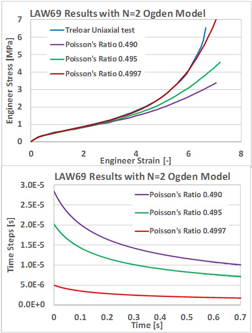
Рисунок 137:

Более высокие значения коэффициента Пуассона могут привести к очень малому временному шагу или расхождению для явных симуляций.

В LAW42 несжимаемость материала обеспечивается с помощью подхода штрафа, который вычисляет давление, пропорциональное изменению плотности.

\[P=K\cdot Fscale_{blk}\cdot\mathrm{f}_{blk}(J)\cdot(J-1) \tag{65}\]

Где,

\(K\) Модуль объемной упругости

\(J=\frac{V}{V_{0}}=\frac{m\rho_{0}}{m\rho}=\frac{\rho_{0}}{\rho}\) Относительный объем, который упрощается до относительной плотности, если масса постоянна

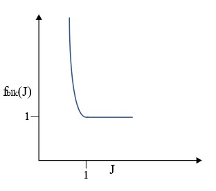
\(\mathrm{f}_{blk}(J)\) Коэффициент масштабирования коэффициента объемной упругости в зависимости от функции относительного объема

\(Fscale_{blk}\) Коэффициент масштабирования абсциссы для функции \(F_{blk}(J)\) Модуль объемной упругости (K) гиперупругих материалов обычно имеет очень высокое значение, которое обеспечивает необходимое сопротивление давлению для поддержания состояния несжимаемости (J=1). Но если материал начинает сжиматься (j < 1), то модуль объемной упругости можно увеличить, включив входную функцию fct_ID^blk, которая позволяет масштабировать значение коэффициента объемной упругости как функцию . По умолчанию масштабирование отсутствует; таким образом, если идентификатор функции равен нулю, а значение функции масштабирования объемной упругости равно 1. Рекомендуется вывести (/ANIM/BRICK/DENS) и просмотреть плотность материала компонентов LAW42, чтобы убедиться, что изменение плотности мало, то есть значение J близко к 1, а материал несжимаем.

width

2.60022in

height

2.30853in

Рисунок 138: Функция масштабного коэффициента модуля объемной упругости fct_ID^blk

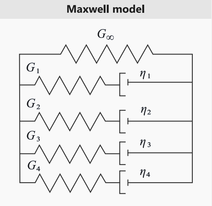
Влияние вязкости (скорости)

Вязкие (скоростные) эффекты моделируются в LAW42 с использованием модели Максвелла, которую можно описать упрощенно как систему \(\eta\) пружин с жесткостью’ \(G_{i}\) и демпферов \(\eta_{i}\):

width

2.60022in

height

2.30853in

Рисунок 139: Модель Максвелла

Модель Максвелла представлена ​​с использованием входных данных ряда Прони (\(G_{i},\tau_{i})\). Гиперупругий начальный модуль сдвига \(\mu\) такой же, как и долгосрочный модуль сдвига \(G_{\infty}\) в модели Максвелла, а \(\tau_{i}\) — это время релаксации:

\[\tau_{i}=\frac{\eta_{i}}{G_{i}} \tag{66}\]

Значения \(G_{i} и \tau_{i}\) должны быть положительными.

/MAT/LAW62 (VISC_HYP)

Закон гипервязкоупругого материала в PRADIOS, который можно использовать для моделирования полимеров и эластомеров.

Гиперупругое поведение в этом материальном законе определяется с помощью следующей функции плотности энергии деформации:

\[W(\lambda_{1},\lambda_{2},\lambda_{3})=\sum_{i=1}^{N}\frac{2\mu_{i}}{\alpha_{i}!}\Big{(}\lambda_{1}\alpha_{i}+\lambda_{2}\alpha_{i}+\lambda_{3}\alpha_{i}-3+ \frac{1}{\beta}(J^{-\alpha_{i}\beta}-1)\Big{)} \tag{67}\]

Где,

\(W\) Плотность энергии деформации

\(\lambda_{i}\) \(i_{th}\) главный stretch

\(J\) Относительный объем, определенный в уравнении 67

\(\beta=\frac{v}{(1-2v)}\)

\(\alpha_{i}\) и \(\mu_{i}\) Пары коэффициентов материальных констант.

Можно определить до 5 пар материальных констант.

Коэффициент Пуассона должен быть (0<v<0,5). Этот закон можно использовать для моделирования сжимаемых или иногда называемых гиперпенистых материалов, задавая низкое значение коэффициента Пуассона.

Примечание: Коэффициенты материала \(\mu_{i}\) различны, но их можно преобразовать с помощью:

\[\mu_{i}^{LAW62}=\frac{\mu_{i}^{LAW42}\cdot a_{i}^{LAW42}}{2} \tag{68}\]

Влияние вязкости (скорости)

Вязкие (скоростные) эффекты моделируются в LAW62 с использованием модели Максвелла, которую можно описать упрощенно как систему из n пружин с жесткостью \(G_{i}\) и демпферов \(\eta_{i}\).

width

2.60022in

height

2.30853in

Рисунок 140: Модель Максвелла

Модель Максвелла представлена ​​с использованием ряда Прони с входными данными. Начальный модуль сдвига равен:

\[G_{0}=\sum_{i=1}^{N}\mu_{i} \tag{69}\]

Сумма \(\mu_{i}\) должна быть больше 0.

\[G_{0}=G_{\infty}+\sum_{i}G_{i} \tag{70}\]

Коэффициент жесткости равен:

\[\gamma_{\infty}=\frac{G_{\infty}}{G_{0}}=1-\sum_{i}\gamma_{i} \tag{71}\]

\[\gamma_{i}=\frac{G_{i}}{G_{0}} \tag{72}\]

С учетом того,

\[\gamma_{i}\in\left[0,\,1\right]\sum_{i}\gamma_{i}<1 \tag{73}и модуль сдвига грунта\]

\[G_{0}=G_{\infty}+\sum_{i}G_{i} \tag{74}\]

Относительное время, \(\tau_{i}\) должно быть положительным:

\[\tau_{i}=\frac{\eta_{i}}{G_{i}} \tag{75}\]

Примечание: Когда вязкость включена, модуль сдвига в LAW62 является начальным модулем сдвига \(G_{0}=\sum_{i=1}^{N}\mu_{i}\), который включает вязкость, но в LAW42 модуль сдвига является долгосрочным модулем сдвига, который не включает вязкость \(G_{\omega}=\frac{\sum_{p=1}^{5}\mu_{p}\cdot a_{p}}{2}\).

/MAT/LAW69

Этот закон, как и /MAT/LAW42 (OGDEN), определяет гиперупругий и несжимаемый материал, заданный с использованием моделей материалов Огдена или Муни-Ривлина. В отличие от LAW42, где параметры материала являются вводными, этот закон вычисляет параметры материала, используя данные испытаний из одноосной инженерной кривой напряжения-деформации.

Этот материал можно использовать с оболочечными и твердыми элементами.

Формулировка плотности энергии деформации, используемая в зависимости от law_ID:

• law_ID = 1 (закон Огдена):

\[W\big{(}\lambda_{1},\lambda_{2},\lambda_{3}\big{)}=\sum_{p=1}^{5}\frac{\mu_{p}}{a_{p}}\big{(}\lambda_{1}a_{p}+\lambda_{2}a_{p}+\lambda_{3}a_{p}-3\big{)}+\frac{K}{2}\big{(}J-1\big{)}^{2} \tag{76}\]

• law_ID = 2 (закон Муни-Ривлина):

\[W=C_{10}\big{(}I_{1}-3\big{)}+C_{0}\big{(}I_{2}-3\big{)} \tag{77}\]

Параметры материала

После считывания кривой напряжения-деформации (fct_ID₁) PRADIOS вычисляет соответствующие пары параметров материала, используя нелинейный алгоритм подгонки наименьших квадратов. Для классического закона Огдена, (law_ID=1), вычисляемые пары параметров материала равны и где значение p определяется через вход N_pair.

Максимальное значение равно N_pair=5 со значением по умолчанию 2. Обычно для хорошего соответствия требуется не более N_pair=3.

Для закона Муни-Ривлина (law_ID =2) параметр материала \(C_{10}\) и \(C_{01}\) рассчитываются для LAW42 Закон Огдена можно рассчитать с помощью этого преобразования:

\(\mu_{1}=2\cdot C_{10},\mu_{2}=-2\cdot C_{01},\alpha_{1}=2 и (\alpha_{2}=)-2\)

Минимальные входные данные испытаний должны представлять собой кривую деформации одноосного растяжения. Если доступны данные одноосного сжатия, то деформация должна монотонно увеличиваться от отрицательного значения при сжатии до положительного значения при растяжении. При сжатии деформация не должна быть меньше -1,0, поскольку деформация -100% физически невозможна.

Для улучшения качества нелинейной подгонки методом наименьших квадратов рекомендуется: - Кривая экспериментальных данных представляет собой гладкую монотонно возрастающую функцию с равномерным распределением точек абсциссы. Количество точек данных на кривой экспериментальных данных должно быть больше количества пар параметров (N_pair).

• Инженерная деформация отрицательна при сжатии и положительна при растяжении. Для данных испытаний на сжатие инженерная деформация должна быть больше -1,0 (максимум 100% сжатия), но также можно использовать данные о деформации только при растяжении.

• Если N_pair ≥ 3, то данные испытаний должны охватывать не менее 100% деформации растяжения и/или 50% деформации сжатия.

• N_pair не следует устанавливать на очень большое значение, чтобы избежать нестабильности в процедуре подгонки.

Этот материальный закон стабилен, когда \(\mu_{p}\alpha_{p}>0\) (при (p)=1,…5) выполняется для пар параметров для всех условий нагрузки. По умолчанию Radios пытается подогнать кривую, учитывая эти условия (\(I_{check}=2)\). Если надлежащее соответствие не может быть найдено, то Radios использует более слабое условие (\(I_{check}=1\):), которое гарантирует, что начальный сдвиг гиперэластичный модуль (\(\mu\)) положительный. Чтобы определить, насколько хорошо рассчитанные параметры материала представляют входные данные испытаний, PRADIOS Starter выводит значение «усредненной ошибки подгонки», которое рекомендуется не превышать 10%. Для визуального сравнения кривая напряжения-деформации, рассчитанная на основе плотности энергии деформации и расчетных параметров материала, также выводится PRADIOS Starter.

Из-за трения, присутствующего в одноосном испытании на сжатие, обычно точнее брать равные данные испытаний на двухосное растяжение и преобразовывать их в одноосные данные сжатия, используя эти формулы ⁷ которые действительны для несжимаемых материалов.

\[\varepsilon_{c}=\frac{1}{\left(\varepsilon_{b}+1\right)^{2}}-1 \tag{78}\]

\[\sigma_{c}=\sigma_{b}\left(1+\varepsilon_{b}\right)^{3} \tag{79}\]

Где,

\(\varepsilon_{c}\) Одноосное инженерное сжатие

\(\varepsilon_{b}\) Равная двухосная инженерная деформация растяжения

\(\sigma_{c}\) Одноосное инженерное напряжение сжатия

\(\sigma_{b}\) Равное двухосное инженерное напряжение растяжения

Несжимаемость материала

Материал LAW69 использует тот же метод для поддержания несжимаемости, что и LAW42. Для получения дополнительной информации см. Коэффициент Пуассона и Несжимаемость материала в LAW42.

Влияние вязкости (скорости)

/VISC/PRONY необходимо использовать с LAW69 для включения вязких эффектов. В качестве альтернативы LAW69 можно использовать для извлечения параметров Огдена или Муни-Ривлина, а затем эти параметры можно использовать в LAW42 с добавленной вязкостью.

/MAT/LAW82

Эта модель материала определяет гиперупругий и несжимаемый материал, указанный с использованием моделей материалов Огдена, Нео-Хукеана или Муни-Ривлина. Этот закон обычно используется для моделирования несжимаемых резин, полимеров, пен и эластомеров.

Этот материал можно использовать с оболочечными и твердыми элементами. По сравнению с LAW42 или LAW62, этот закон использует другую формулировку плотности энергии деформации Огдена, приведенную в уравнении 80. Формулировка плотности энергии деформации LAW82 соответствует той, которая используется в гиперупругой модели некоторых других решателей конечных элементов и, таким образом, параметры материала для этой формы плотности энергии деформации Огдена иногда доступны у поставщиков материалов или из других источников.

\[W=\sum_{i=1}^{N}\frac{2\mu_{i}}{\alpha_{i}^{2}}\big{(}\overline{\lambda}_{i}\alpha_{i}+\overline{\lambda}_{2}\alpha_{i}+\overline{\lambda}_{3}\alpha_{i}-3\big{)}+\sum_{i=1}^{N}\frac{1}{D_{i}}\big{(}J-1\big{)}_{2i} \tag{80}\]

Где,

\(W\) Плотность энергии деформации

\(N\) Количество материальных констант \(\alpha_{i},\mu_{i}\) и \(D_{i}\)

\(\overline{\lambda}_{i}=J^{\frac{1}{3}}\lambda_{i}\) Девиаторное растяжение

\(J\) Относительный объем, как определено в уравнении 56

Начальный модуль сдвига:

\[\mu=\sum_{i=1}^{N}\mu_{i} \tag{81}\]

Модуль объемной упругости рассчитывается как \(K=\frac{2}{D_{1}}\) на основе этих правил:

• Если \(v=0\), следует ввести \(D_{1}\).

• Если \(v\neq 0\), вход \(D_{1}\) игнорируется и будет пересчитан и выведен в выход Starter с использованием:

\[D_{1}=\frac{3(1-2v)}{\mu(1+v)} \tag{82}\]

• Если \(v=0\) и \(D_{1}\) =0, используется значение по умолчанию \(v=0.475\) и \(D_{1}\) вычисляется с использованием уравнения 82

Модель Нео-Хукена

Как и LAW42, LAW82 также можно упростить до модели Нео-Хукена с использованием:

\(\mu_{1}=2\cdot C_{10},\alpha_{1}=2) и \mu_{2}=\alpha_{2}=0\)

Модель Муни-Ривлина

Как и LAW42, LAW82 также можно упростить до модели Муни-Ривлина, используя:

\(\mu_{1}=2\cdot C_{10},\mu_{2}=2\cdot C_{01},\alpha_{1}=2 и \alpha_{2}=-2\)

Вязкие (скоростные) эффекты

``/VISC/PRONY``необходимо использовать с LAW82 для включения вязких эффектов.

Проверка устойчивости по условию Дрюкера

В LAW42 и LAW69 устойчивость по Дрюкеру автоматически вычисляется PRADIOS Starter.

Условие устойчивости по Дрюкеру проверяет, удовлетворяет ли изменение напряжения Кирхгофа, соответствующее бесконечно малому изменению логарифмической деформации (истинной деформации), следующему неравенству.

Где, i =1,2,3 главное направление.

При изменении логарифмической деформации

\[de_{i}=\frac{d\lambda_{i}}{\lambda_{i}} \tag{84}\]

\(d\tau_{i}=J\cdot d\sigma_{i}\) Изменение напряжения Кирхгофа

\(d\tau=\mathbf{D}:d\varepsilon\) Соотношение между напряжением Кирхгофа и логарифмической деформацией

Условие устойчивости Дрюкера будет:

\[\sum d\varepsilon :\mathbf{D}:d\varepsilon > 0 \tag{85}\]

Здесь \(\mathbf{D}\) — матрица тангенциальной жесткости материала, а также наклон кривой напряжения-деформации:

\[\tag{86}\]

\[\begin{split}\mathbf{D} =\left [ \begin{matrix} D_{11}&D_{12}&D_{13} \\ D_{21}&D_{22}&D_{23} \\ D_{31}&D_{32}&D_{33} \end{matrix}\right]\end{split}\]

Для стабильного материала требуется, чтобы тангенциальная жесткость материала \(\mathbf{D}\) была положительной (наклон кривой напряжения-деформации положительный). Тангенциальная матрица материала \(\mathbf{D}\) положительна, если выполняются следующие условия:

\[I_{1}=tr(\mathbf{D})=D_{11}+D_{22}+D_{33}>0 \tag{87}\]

\[I_{2}=D_{11}D_{22}+D_{22}D_{33}+D_{33}D_{11}-D_{23}-D_{13}{}^{2}-D_{12}{}^{2}>0 \tag{88}\]

\[I_{3}=\det(\mathbf{D}`)>0 \tag{89}\]

Напряжение Кирхгофа для модели Огдена равно:

\[\tau_{i}=\sum_{p}\mu_{R}\Big{[}\overline{\lambda}_{\alpha p}-\frac{1}{3}\big{(}\overline{\lambda}_{I,p}+\overline{\lambda}_{2,p}+\overline{\lambda}_{3,p}\big{)}\Big{]}+K\big{(}J^{2}-J\big{)}\]

Поскольку \(D_{ij}=\frac{\partial\tau_{i}}{\partial\lambda_{j}}\), тогда для заданного параметра Огдена \(\alpha_{p}\), \(\mu_{p}\) с условиями \(I_{1}>0, I_{2}>0 и I_{3}>0\), тогда можно было бы рассчитать диапазон деформации материала в стабильности по Друкеру. .. image:: vertopal_75794439f47d439ba01f734ac3f4dcc1/media/image-10.jpg

width

6.65882in

height

5.00868in

Рисунок 141:

Критерий стабильности Дрюкера вычисляет диапазон деформаций, при которых модель материала останется стабильной, исходя из заданных параметров материала. Эта проверка стабильности не может быть выполнена для каждой деформации, однако обычно её используют для оценки стабильности материала при однолучевой, двулучевой и плоскостной нагрузке.

Например, при использовании следующих параметров Огдена:

:math:mu_{1} = 13.99077258830 :math:alpha_{1} = 3.78819292935039

:math:mu_{2} = 9.13454532223 :math:alpha_{2} = 7.17617341059

:math:mu_{3} = 8.904655103235 :math:alpha_{3} = 7.27028137148

Тогда проверка стабильности Дрюкера будет автоматически выполнена в PRADIOS Starter, и результаты будут выведены в файл вывода Starter *0.out. В нем показывается деформация, при которой может возникнуть нестабильность для заданных параметров Огдена:

CHECK THE DRUCKER PRAGER STABILITY CONDITIONS
       -----------------------------------------------
     MATERIAL LAW = OGDEN (LAW42)
     MATERIAL NUMBER = 1
      TEST TYPE = UNIXIAL
       COMPRESSION:   UNSTABLE AT A NOMINAL STRAIN LESS THAN -0.3880000000000
       TENSION:       UNSTABLE AT A NOMINAL STRAIN LARGER THAN 0.9709999999999
      TEST TYPE = BIAXIAL
       COMPRESSION:   UNSTABLE AT A NOMINAL STRAIN LESS THAN -0.2880000000000
       TENSION:       UNSTABLE AT A NOMINAL STRAIN LARGER THAN 0.2780000000000
      TEST TYPE = PLANAR (SHEAR)
       COMPRESSION:   UNSTABLE AT A NOMINAL STRAIN LESS THAN -0.3680000000000
       TENSION:       UNSTABLE AT A NOMINAL STRAIN LARGER THAN 0.5829999999999

Примечание: Для материала Нео-Хука с \(C_{10}!>!0 (or \mu_{1}!>!0)\), материал всегда является стабильным, и критическое значение не определяется проверкой стабильности по Друкеру.

Для материала Мунни-Ривлина необходимо проверить стабильность по Друкеру, так как параметры \(C_{01} or \mu_{2}\) ​ могут быть отрицательными, что ведет к нестабильности материала.

/MAT/LAW88

Этот закон использует табличные данные испытаний на однолучевое растяжение и сжатие с инженерским напряжением и деформацией при различных скоростях деформации для моделирования несжимаемых материалов. Он совместим только с твердыми элементами.

Материал основан на следующей функции энергии деформации Огдена, при этом не требуется подгонка кривых для извлечения констант материала, как в большинстве других гиперэластичных моделей. :sup:8

\[W=\sum_{i=1}^{3}\sum_{j=1}^{m}\frac{\mu_{j}}{\alpha_{j}}\Big{(}\lambda_{i}\alpha_{j}-1\Big{)}+{K(J-1-\ln J)} \tag{91}\]

Вместо этого данный закон определяет функцию Огдена непосредственно из табличных данных кривой напряжение-деформация при однолучевом растяжении.

В отличие от других законов Огдена, модуль объема (Bulk Modulus) должен быть введен либо из экспериментальных данных, либо извлечен из результатов в Starter по кривой Огдена LAW69. При сравнении результатов между LAW42 или LAW69 и LAW88 необходимо использовать один и тот же модуль объема.

Поведение при разгрузке

Разгрузка может быть представлена с помощью функции разгрузки или путем задания гистерезиса и фактора формы в модели повреждения, основанной на энергии.

Если используется модель повреждения, кривые нагружения применяются как для загрузки, так и для разгрузки, а тензор напряжений при разгрузке уменьшается по формуле:

\[\sigma=\big{(}1-D\big{)}\sigma \tag{92}\]

где

\[D=\big{(}1-Hys)\bigg{(}1-\bigg{(}\frac{W_{cur}}{W_{\max}}\bigg{)}^{Shape}\bigg{)} \tag{93}\]

Здесь,

:math:W_{cur} — текущая энергия

:math:W_{max} — максимальная энергия, соответствующая квазистатическому поведению

Hys и Shape — параметры, заданные пользователем

Если предоставлена кривая разгрузки, доступны следующие опции:

Растяжение Загрузка и разгрузка

= 0

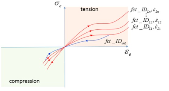
*Рисунок 142:

При загрузке используется функция загрузки fct_ID^Li

При разгрузке используется функция разгрузки fct_ID^unL

= 1

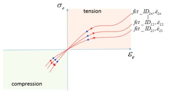
Рисунок 143:

При загрузке и разгрузке используется одна и та же функция fct_ID^Li

= -1

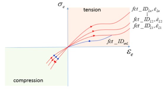
width

5.20833in

height

2.79878in

Рисунок 144:

При использовании функции загрузки fct_ID^Li для растяжения

• Растяжение (Тension)

Разгрузка использует функцию разгрузки fct_ID^unL

• Сжатие

Разгрузка использует загрузку fct_ID^Li

Вязкость (Эффекты скорости

Эффекты скорости деформации можно смоделировать, включив данные испытаний на инженерное напряжение деформации при различных скоростях деформации. Это может быть проще, чем расчет параметров вязкости для традиционных моделей гиперупругого материала.

Вывод

Обязательно используйте закон материала, который наилучшим образом соответствует имеющимся данным испытаний.

Например, если доступны минимальные данные испытаний и деформации не слишком велики, можно использовать модель LAW42 NeoHookean. Если известно состояние нагрузки, важно иметь данные испытаний, которые представляют это состояние напряжения, и убедиться, что модель материала соответствует этим данным испытаний.

1. Ogden, R. W., and Non-linear Elastic Deformations. “Ellis Horwood”. Нью-Йорк (1984)

2. Miller, Kurt. “Testing Elastomers for Hyperelastic Material Models in Finite Element Analysis” Axel Products, Inc., Энн-Арбор, Мичиган (2017). Последнее изменение 5 апреля 2017 г.

Arruda-Boyce (/MAT/LAW92)

LAW92 описывает модель материала Арруды-Бойса, которую можно использовать для моделирования гиперупругого поведения. Эта модель основана на статистической механике материала с кубическим репрезентативным элементом объема, содержащим восемь цепей вдоль диагональных направлений.

Она предполагает, что молекулы цепи расположены в среднем вдоль диагоналей кубического в основном пространстве растяжения.

Параметры материала

Функция плотности энергии деформации:

\[W=\mu\sum_{l=1}^{5}\frac{c_{i}}{(\lambda_{m})^{2i-2}}({l_{1}^{i}}-3^{i})+\frac{1}{D}\big{(}\frac{J^{2}-1}{2}+\ln(J)\big{)} \tag{94}\]

Константа материала, \(c_{i}\) являются:

\(c_{1}=\frac{1}{2}, c_{2}=\frac{1}{20}, c_{3}=\frac{11}{1050}, c_{4}=\frac{19}{7000}, c_{5}=\frac{519}{673750}\)

\(\overline{I_{1}}=\overline{\lambda_{1}^2}+\overline{\lambda_{2}^2}+\overline{\lambda_{3}^2}\) Первый инвариант деформации

\(\lambda_{i}\) \(i_{th}\) основное инженерное растяжение

Материал с LAW92 можно определить двумя способами:

• Ввод параметров

Модуль сдвига, объемный модуль и растяжение при деформации (\(\mu,D,\lambda_{m})\)

Где только вышеуказанные 3 параметра с ясным физическим смыслом необходимы для определения материала.

\(\mu\) — это модуль сдвига при нулевой деформации.

\[D=\frac{2}{K} \tag{95}\]

Где,

\(K\) Коэффициент объемной деформации при нулевой деформации

\(\lambda_{m}\) Определяет предел растяжения

7. Axel Products, Inc. “Сжатие или двуосное расширение”, Ann Arbor, MI (2017). Последнее изменение 12 ноября 2008 г.

8. Kolling, S., P. A. Du Bois, D. J. Benson и W. W. Feng. “Табличная формулировка гиперэластичности с эффектами скорости и повреждениями”. Computational Mechanics 40, № 5 (2007): 885-899

   Также называется фиксирующим растяжением. Определяет начало фазы затвердевания при растяжении

   (фиксирующая деформация при растяжении). По умолчанию = 7,0.

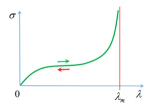
Рисунок 145:блокировка растяжения \(\lambda_{m}\)

При параметрическом вводе коэффициент Пуассона вычисляется как:

\[v=\frac{3K-2\mu}{6K+2\mu} \tag{96}\]

• При использовании ввода функции необходимо определить коэффициент Пуассона и Itype. Itype определяет, какой тип данных испытания на деформацию при проектировании используется в качестве входных данных.

width

2.93342in

height

2.46679in

Рисунок 146: Itype = 1: одноосный тест данных .. image:: vertopal_75794439f47d439ba01f734ac3f4dcc1/media/image1-7.jpg

width

2.73349in

height

2.01675in

Рисунок 147: Itype = 2: Тест данных для эквибиаксиального сжатия

Рисунок 148: Itype = 3: Тест плоских данных

Коэффициент Пуассона и несжимаемость материала

Если входные данные функции определены, то параметры \(\mu,D,\lambda_{m}\) игнорируются, и PRADIOS вычислит постоянную материала, подгоняя входную функцию. Для подгонки параметров ArrudaBoyce PRADIOS использует нелинейный алгоритм наименьших квадратов. Подгонка кривой выполняется с использованием предположения, что значение Пуассона близко к 0,5, что означает, что материал несжимаем. Подобно другим моделям гиперупругих материалов, значения коэффициента Пуассона, близкие к 0,5, приводят к высокому модулю объемной упругости и меньшему временному шагу. Для хорошего баланса между несжимаемостью и разумным временным шагом рекомендуется значение коэффициента Пуассона 0,495.

Информацию о подгонке материалов можно найти в выходном файле Starter (*0000.out).

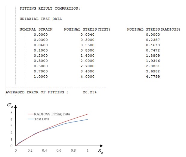
Рисунок 149: пример функции LAW92

Ошибка подгонки и параметры подогнанного материала печатаются в выходном файле Starter.

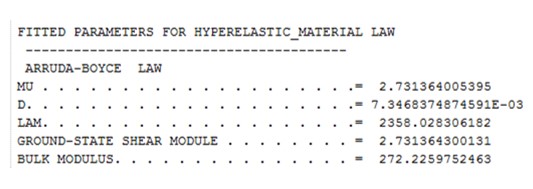
Рисунок 150:*

Вязкость (Эффекты скорости

/VISC/PRONY необходимо использовать с LAW92 для включения эффектов вязкости.

Йео (/MAT/LAW94)

LAW94 — это гиперупругая модель материала, которую можно использовать для описания несжимаемых материалов.

Функция плотности энергии деформации LAW94 зависит только от первого инварианта деформации и вычисляется как:

\[W=\sum_{i=1}^3\left[C_{i0}(I_{i}-3)^i+\frac{1}{D_{i}}(J-1)^2i\right] \tag{97}\]

Где,

\(\overline{I_{1}}=\overline{\lambda_{1}^2}+\overline{\lambda_{2}^2}+\overline{\lambda_{3}^2}\) Первый инвариант деформации

\(\overline{\lambda_{i}}=J^{-\frac{1}{3}}\lambda_{i}\) Девиаторное растяжение

Напряжение Коши равно:

\[\sigma_{i}=\frac{\lambda_{i}}{J}\frac{\partial W}{\partial\lambda_{i}}\]

Параметры материала

Для несжимаемых материалов с =1 только и являются входными данными, а модель Йео сводится к модели НеоХука.

9. Arruda, E. M. и Boyce, M. C., 1993, «Трехмерная модель для поведения эластичных резиновых материалов при больших растяжениях», J. Mech. Phys. Solids, 41(2), стр. 389–412

\(C_{10}C_{20}C_{30}\) Константы материала определяют девиаторную часть (изменение формы) материала

\(D_{1,}D_{2,}D_{3}\) Параметры определяют объемное изменение материала

Эти шесть констант материала необходимо рассчитать с помощью подгонки кривой данные испытаний материала. RD-E: 5600

Гиперупругий материал с вводом кривой включает подгонку Йео Скрипт Compose для одноосных данных испытаний. Модель материала Йео была показана для моделирования всех моделей деформации, даже если подгонка кривой была получена с использованием только данных одноосных испытаний.

Начальный модуль сдвига и объемный модуль упругости:

\[\mu=2\cdot C_{10} \tag{99}\]

и

\[K=\frac{2}{D_{1}} \tag{100}\]

Коэффициент Пуассона и несжимаемость материала

LAW94 доступен только как модель несжимаемого материала.

Если = D₁ 0, то рассматривается несжимаемый материал, где v = 0,495 D₁ вычисляется как:

\[D_{1}=\frac{3(1-2\nu)}{\mu(1+\nu)} \tag{101}\]

Бергстрем-Бойс (/MAT/LAW95)

Этот закон является конститутивной моделью для прогнозирования нелинейной зависимости от времени эластомерных материалов. Он использует полиномиальную модель материала для гиперупругого реакции материала и модель материала Бергстрема-Бойса для представления нелинейной вязкоупругой, зависящей от времени реакции материала.

Этот закон совместим только с твердыми элементами.

Реакция материала может быть представлена ​​с помощью двух параллельных сетей A и B. Сеть A является равновесной сетью с нелинейным гиперупругим компонентом. В сети B нелинейный гиперупругий компонент находится последовательно с нелинейным вязкоупругим элементом потока, и, следовательно, является сетью, зависящей от времени.

10. Yeoh, O. H. “Некоторые формы функции энергии деформации для резины”. Rubber Chemistry and technology 66, № 5 (1993): 754-771 .. image:: vertopal_75794439f47d439ba01f734ac3f4dcc1/media/image2-1.png

width

3.45667in

height

3.48333in

Рисунок 151:

Параметры материала

Та же полиномиальная формулировка плотности энергии деформации используется для гиперупругих компонентов в обеих сетях. В сети B она масштабируется на коэффициент S_b. Затем плотность энергии деформации записывается для гиперупругого компонента сети.

\[W_{A}=\sum_{i+j=1}^{3}C_{ij}\big{(}I_{1}-3\big{)}^i\cdot\big{(}I_{2}-3\big{)}^J+\sum_{i=1}^{3}\frac{1}{D_{i}}(J-1)^2i \tag{102}\]

и

\[W_{B}=S_{b}\cdot W_{A} \tag{103}\]

Где,

\(\overline{I_{1}}=\overline{\lambda_{1}^2}+\overline{\lambda_{2}^2}+\overline{\lambda_{3}^2}\)

\(\overline{I_{2}}=\overline{\lambda_{1}^{-2}}+\overline{\lambda_{2}^{-2}}+\overline{\lambda_{3}^{-2}}\)

\(\overline{\lambda_{i}}=J^{-\frac{1}{3}}\lambda_{i}\)

\(C_{ij}\) и \(D_{i}\) Параметры материала

Гиперупругий компонент напряжения Коши вычисляется как:

\[\sigma_{i}=\frac{\dot{\lambda}_{i}}{J}\frac{\partial W}{\partial\dot{\lambda}_{i}} \tag{104}\]

Общее напряжение — это сумма напряжений в сети A и сети B.

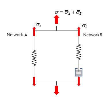
Рисунок 152:

\(\overline{\sigma}=\overline{\sigma_{A}}+\overline{\sigma_{B}}\)

Поскольку \(W_{B}=S_{b}\cdot W_{A}\), то \(\overline{\sigma}_{B}=S_{b}\cdot\overline{\sigma}_{A}\) и общее напряжение равно \(\sigma=(1+S_{b})\cdot\overline{\sigma}_{A}\)

Например, в одном испытании на растяжение. Если использовать S_b, то напряжение в 3 раза больше, чем без учета вязкости (что означает только учет гиперупругости).

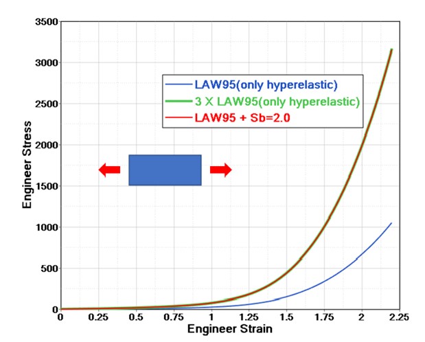
Рисунок 153:

Для специальных значений полиномиальная модель может быть сведена к следующим материальным моделям.

• Yeoh:

*J*=0

Где, \(C_{10,}C_{20,}C_{30,}\) не равны нулю.

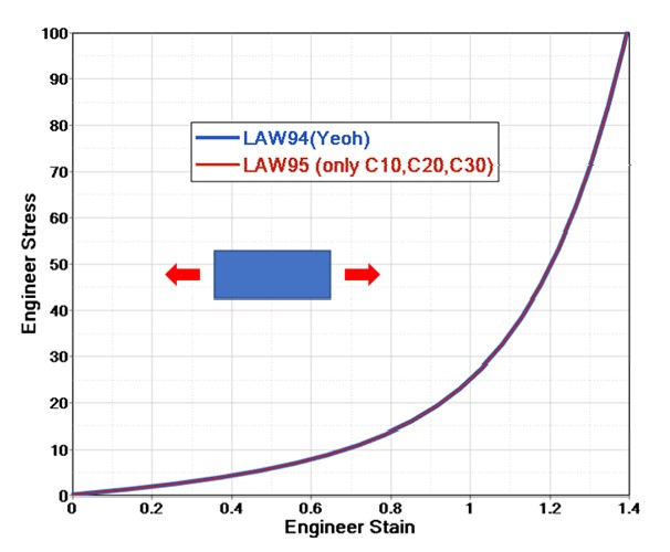
Рисунок 154:

• Mooney-Rivlin:

\(i+j=1\)

Где, \(C_{10}\) и \(C_{01}\) не равны нулю и \(D_{2}=D_{3}=0.\)

• Neo-Hookean:

Только \(C_{10}\) и \(D_{1}\) не равны нулю.

Где,

\(C_{ij}\) и \(D_{i}\) Параметры материала, которые можно рассчитать, выполнив подгонку кривой для данных квазистатических испытаний материалов.

RD-E: 5600 Гиперупругий материал с вводом кривой, содержит пример подгонки кривой для моделей материалов Муни-Ривлина и Йео. можно рассчитать из объемного модуля или оставить пустым.

Начальный модуль сдвига и объемный модуль вычисляются как:

\[\mu=2\big{(}S_{b}+1\big{)}\big{(}C_{10}+C_{01}\big{)} \tag{105}\]

и

\[K=\frac{2}{D_{1}}\big{(}1+S_{b}\big{)} \tag{106}\]

Если объемный модуль материала известен, можно рассчитать D₁, или если D₁ =0, предполагается несжимаемый материал.

Эффекты вязкости (скорости)

Эффективная скорость деформации ползучести в сети B определяется по формуле:

\[\dot{\varepsilon}_{B}^{\nu}=A(\overline{\dot{\lambda}}-1+\dot{\varepsilon}g)^{C}\frac{\overline{\sigma}_{B}}{\tau_{ref}}^{M} \tag{107}\]

Где,

\(\overline{\dot{\lambda}}=\sqrt{\frac{T_{1}}{3}}\)

\(\overline{\sigma}_{B}\) Эффективное напряжение в сети B.

\(A, \bar{\varepsilon}, M, C\) , and \(\tau_{ref}\) Входные параметры материала. Константы материала A, M и C ограничены определенным диапазоном действительных значений, как определено в Справочном руководстве. Если доступны ограниченные данные, можно использовать метод проб и ошибок¹¹ для определения этих констант. Начните со значений по умолчанию \(\bar{\xi}, M, C, S_{b}\) =1,6; и A=5. Затем сравните прогнозы модели с экспериментальными данными по крайней мере для одной скорости деформации и скорректируйте A, чтобы получить соответствие для данных скорости деформации.

11. Bergström, J. S., and M. C. Boyce. “Constitutive modeling of the large strain time-dependent behavior of elastomers.” Journal of the Mechanics and Physics of Solids 46, no. 5 (1998): 931-954

Эласто-пластичные материалы

Джонсон-Кук (/MAT/LAW2)

В LAW2 расчет напряжений состоит из трех частей.

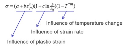
Рисунок 155: - Влияние пластической деформации

• Влияние скорости деформации

• Влияние изменения температуры

Параметры материала

Существует два способа ввода параметра материала для LAW2.

• Iflag=0: Классический ввод для параметра Джонсона-Кука a, b, n активен

• Iflag=1: Новый, упрощенный ввод с пределом текучести, UTS (инженерное напряжение) или деформацией при UTS Iflag= 0

\[\sigma=a+b\cdot\varepsilon_{pn} \tag{108}\]

Где,

a

Предел текучести, который можно определить по результатам испытания материала и преобразовать в истинное напряжение.

b и n

Параметры материала. Подгонка кривой напряжения-деформации материала (например, скрипт Laduga Compose) может привести к этим двум параметрам.

Iflag = 1

С этим новым вводом вам понадобится предел текучести, предел прочности на растяжение (UTS) и инженерная деформация в точке сужения. С этим новым вводом PRADIOS автоматически вычисляет эквивалентное значение для a, b и n.

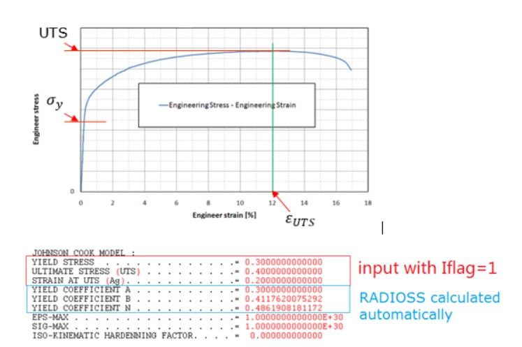
Рисунок 156: Испытание на растяжение

Скорость деформации

Скорость деформации оказывает большое влияние на характер материала на характеристики удара при растяжении или при разрыве. В теории Джонсона-Кука предел текучести напрямую зависит от скорости деформации и описывается как:

\[\sigma=\left(a+b\cdot\varepsilon_{p\eta}\right)\left(1+c\ln\frac{\xi}{\xi_{0}}\right) \tag{109}\]

Обычно предел текучести увеличивается с увеличением скорости деформации испытания. С коэффициентом скорости деформации c вы можете масштабировать фактор увеличения предела текучести. Никакого влияния скорости деформации также не может быть определено, если c =0; или с \(\xi_{0}=10^{30} или \xi\leq\xi_{0}).\) .. image:: vertopal_75794439f47d439ba01f734ac3f4dcc1/media/image27.jpg

width

2.9836in

height

3.0836in

Рисунок 157:

Изменение температуры

Предел текучести уменьшается с ростом температуры. В LAW2 влияние рассматривается с \(\left(1-T^{\*m}\right).\)

\[\sigma=\left(a+b\cdot\varepsilon_{p}n\right)\left(1+c\ln\frac{\dot{\varepsilon}}{\dot{\varepsilon}_{0}}\right)\left(1-T^{\*m}\right) \tag{110}\]

с

\[T^{\*}=\frac{T-T_{r}}{T_{melt}-T_{r}} \tag{111}\]

Где,

\(T_{melt}\) Температура расплава в единицах Кельвина.

\(T_{r}\) Температура в помещении в единицах Кельвина.

С T, вычисленным как:

\[T=T_{i}+\frac{E_{int}}{\rho C_{p}\left(Volume\right)} \tag{112}\]

Где,

\(E_{int}\) Внутренняя энергия.

Изменение внутренней энергии повлияет на предел текучести в законе Джонсона-Кука.

Коэффициент упрочнения

Металл деформируется до предела текучести, а затем в целом закаляется (предел текучести увеличивается). Разные материалы демонстрируют разные способы закалки (изотропная закалка, кинематическая закалка и т. д.). Это также очень важная характеристика материала (для упругого возврата).

В LAW2 используйте опцию \(C_{hard}\) (коэффициент закалки), чтобы описать, какая модель закалки используется для материала. Эта функция также доступна в материалах LAW36, 43, 44, 57, 60, 66, 73 и 74.

Значение \(C_{hard}\) составляет от 1 до 0. \(C_{hard}\) =0 для изотропной модели, \(C_{hard}\) =1 для кинематической модели Прагера-Циглера или между 1 и 0 для закалки между двумя указанными выше моделями.

\(C_{hard}\) = 0: Изотропная модель

В одномерном случае материал укрепляется после предела текучести.

Максимальное напряжение последнего растяжения является пределом текучести при последующей нагрузке, и этот новый предел текучести одинаков при последующих растяжении и сжатии.

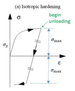
Рисунок 158:

\(C_{hard}\) = 1: Кинематическая модель Прагера-Циглера

Для моделирования эффекта Баушингера (после упрочнения при растяжении происходит размягчение при последующем сжатии, что означает снижение текучести при сжатии) используйте кинематическое упрочнение.

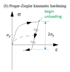
Рисунок 159:

Упругий пластичный кусочно-линейный материал (/MAT/LAW36)

В LAW36 количество пластических кривых напряжения-деформации можно определить напрямую для различных скоростей деформации.

Пластическое напряжение-деформация высокой скорости деформации всегда должно быть выше нижней пластической кривой напряжения-деформации. .. image:: vertopal_75794439f47d439ba01f734ac3f4dcc1/media/image30.jpg

width

8.05061in

height

3.04185in

Рисунок 160:

Модуль Юнга

Модуль Юнга можно обновить (уменьшить) при разгрузке с помощью опций fct_ID_E, E_inf и C_E. Использование этой функции повышает точность пружинения (в фазе разгрузки) для высокопрочной стали. Эта функция также доступна в материалах LAW43, LAW57, LAW60, LAW74 и LAW78.

• Используйте fct_ID_E для обновления модуля Юнга (fct_ID_E ≠ 0):

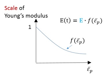
Рисунок 161:

• Используйте E_inf and CE обновить модуль Юнга (fct_ID_E = 0):

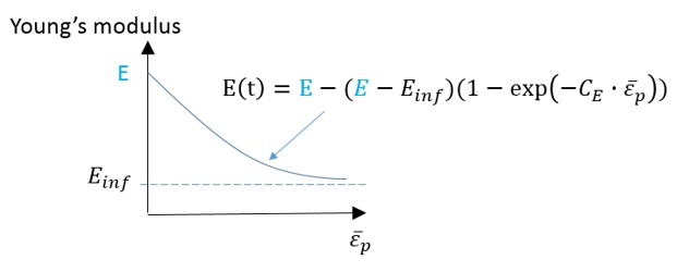
Рисунок 162:

Поведение материала

fct_ID_p используется для различения поведения при растяжении и сжатии для определенных материалов (текучесть, зависящая от давления). Затем эффективный предел текучести получается путем умножения номинального предела текучести на коэффициент текучести, соответствующий фактическому давлению.

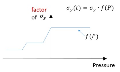
Рисунок 163:

См. также

/MAT/LAW2 (PLAS_JOHNS) (Starter)

RD-E: 1101 Elasto-plastic Material Law Characterization

Материалы HILL

В законах о материалах PRADIOS LAW32, LAW43, LAW72, LAW73, LAW74, LAW78 и LAW93 используются критерии HILL.

Критерии ХИЛЛА

Типичные критерии ХИЛЛА:

• 3D эквивалентное напряжение ХИЛЛА:

\[f=\sqrt{F\big{(}\sigma_{yy}-\sigma_{zz}\big{)}^{2}+G\big{(}\sigma_{zz}-\sigma_{xx}\big{)}^{2}+H\big{(}\sigma_{xx}-\sigma_{yy}\big{)}^{2}+2L\sigma_{yz}^{2}+2M\sigma_{xx}^{2}+2N\sigma_{xy}^{2}} \tag{113}\]

\[=\sqrt{(G+H)\sigma_{xx}^{2}+(F+H)\sigma_{yy}^{2}+(F+G)\sigma_{zz}^{2}-2H\sigma_{xx}\sigma_{yy}-2F\sigma_{yy}\sigma_{zz}-2G\sigma_{zz}\sigma_{xx}+2L\sigma_{yz}^{2}+2M\sigma_{xx}^{2}+2N\sigma_{xy}^{2}}\]

• Элемент оболочки:

\[f=\sqrt{F\sigma_{yy}^{2}+G\sigma_{xx}^{2}+H\big{(}\sigma_{xx}-\sigma_{yy}\big{)}^{2}+2N\sigma_{xy}^{2}}=\sqrt{(G+H)\sigma_{xx}^{2}+(F+H)\sigma_{yy}^{2}-2H\sigma_{xx}\sigma_{yy}+2N\sigma_{xy}^{2}} \tag{114}\]

Где F, G, H, L, M и N — шесть анизотропных ХИЛЛ параметры. Для элементов оболочки только F, G, H и N являются четырьмя необходимыми параметрами HILL.

В LAW78 критерии HILL следующие:

\[\varphi(A)=\frac{1}{G+H}\cdot A_{xx}^{2}-\frac{2r_{0}}{\frac{1+r_{0}}{2H}}A_{xx}A_{yy}+\frac{r_{0}(1+r_{90})}{\frac{r_{90}(1+r_{0})}{F+H}}A_{yy}^{2}+\frac{r_{0}+r_{90}}{\frac{r_{90}(1+r_{0})}{2N}}A_{xy}^{2} \tag{115}\]

Существует два способа определения параметров HILL с использованием параметров Лэнкфорда.

◦ Коэффициент деформации \(r_{00}, r_{45}, r_{90}\) (LAW32, LAW43, LAW72, LAW73)

◦ Коэффициент текучести \(R_{1}, R_{22}, R_{33}, R_{12}, R_{13}, R_{23}\) (LAW74, LAW93)

Коэффициент деформации

Параметры Ланкфорда \(r_{\alpha}\) — это отношение пластической деформации в плоскости и пластической деформации в направлении толщины \(\varepsilon_{33}\).

\[r_{\alpha}=\frac{d\varepsilon_{\alpha\neq 2}}{d\varepsilon_{33}} \tag{116}\]

Где, \(\alpha\) — угол к ортотропному направлению 1.

\(r_{\alpha}\) можно измерить с помощью разных образцов, которые разрезаны под разным углом к ​​ортотропному направлению 1. Например, \(r_{00}\) измерено при испытании на растяжение, в котором направление нагрузки вдоль ортотропного направления 1. \(r_{90}\) измерено при испытании на растяжение, в котором нагрузка перпендикулярна ортотропному направлению 1.

Отношение деформации — это деформация в направлении ширины образца к деформации в направлении толщины образца. .. image:: vertopal_75794439f47d439ba01f734ac3f4dcc1/media/image3-5.jpg

width

4.9921in

height

2.32521in

Рисунок 164: В этом случае параметры HILL следующие:

\[F=\frac{r_{00}}{r_{90}(r_{00}+1)} \tag{117}\]

\[G=\frac{1}{(r_{00}+1)} \tag{118}\]

\[H=\frac{r_{00}}{(r_{00}+1)} \tag{119}\]

\[N=\frac{(1+2r_{45})(r_{00}+r_{90})}{2r_{90}(r_{00}+1)} \tag{120}\]

Здесь *G+H*=1.

В LAW32, LAW43 и LAW73 критерии HILL следующие:

\[\sigma_{eq}=\sqrt{A_{1}\sigma_{1}^{2}+A_{2}\sigma_{2}^{2}-A_{3}\sigma_{1}\sigma_{2}+A_{1}\sigma_{12}^{2}} \tag{121}\]

\(R=\frac{r_{00}+2r_{4.5}+r_{90}}{4}\) \(H=\frac{R}{1+R}\)

\(A _{1}=H\Big{(}1+\frac{1}{r_{00}}\Big{)}\) \(A_{2}=H\Big{(}1+\frac{1}{r_{90}}\Big{)}\)

\(A_{3}=2H\) \(A_{12}=2H(r_{4.5}+0.5)\Big{(}\frac{1}{r_{00}}+\frac{1}{r_{90}}\Big{)}\)

Все они запрашивают параметр Ланкфорда (коэффициент деформации) \(r_{00}, r_{4.5}, r_{90}\) и параметр HILL \(A_{i}\) автоматически вычисляется PRADIOS.

Коэффициент текучести

В LAW93 используется отношение предела текучести:

\[R_{ij}=\frac{\sigma_{ij}}{\sigma_{0}} \tag{122}\]

Чтобы получить отношение предела текучести \(R_{ij}\), необходимо измерить предел текучести в двух случаях нагрузки.

• Предел текучести \(\sigma_{11,}\sigma_{22,}\sigma_{33}\) из испытания на растяжение

• Предел текучести при сдвиге \(\sigma_{12,}\sigma_{13,}\sigma_{23}\) из испытания на сдвиг

В LAW93, если используется ввод параметров, то возьмите начальный параметр напряжения \(\sigma_{y}\) в качестве опорного предела текучести \(\sigma_{0}\). Если используется входная кривая, то возьмите предел текучести из кривой в качестве опорного предела текучести \(\sigma_{0}\).

Четыре параметра HILL для оболочки автоматически вычисляются PRADIOS.

\[F=\frac{1}{2}(\frac{1}{R_{22}^{2}}+\frac{1}{R_{33}^{2}}\frac{1}{R_{11}^{2}}) \tag{123}\]

\[H=\frac{1}{2}(\frac{1}{R_{22}^{2}}+\frac{1}{R_{11}^{2}}-\frac{1}{R_{33}^{2}}) \tag{124}\]

\[\tag{125}\]

\[N=\frac{3}{2R_{12}^{2}} \tag{126}\]

В LAW74 коэффициент текучести \(R_{ij}\) используется с пределом текучести \(\sigma_{11,}\sigma_{22,}\sigma_{33,}\) и \(\sigma_{12,}\sigma_{13}\sigma_{23}\) вводимыми напрямую, а затем шесть параметров HILL для твердого тела автоматически вычисляются PRADIOS.

\(F=\frac{1}{2}\Bigg{(}\frac{1}{\sigma_{22}^{2}}+\frac{1}{\sigma_{33}^{2}}-\frac{1}{\sigma_{11}^{2}}\Bigg{)}\) \(G=\frac{1}{2}\Bigg{(}\frac{1}{\sigma_{22}^{2}}+\frac{1}{\sigma_{33}^{2}}-\frac{1}{\sigma_{11}^{2}}\Bigg{)}\)

\(H=\frac{1}{2}\Bigg{(}\frac{1}{\sigma_{22}^{2}}+\frac{1}{\sigma_{33}^{2}}-\frac{1}{\sigma_{11}^{2}}\Bigg{)}\) \(L=\frac{1}{2\sigma_{23}^{2}}\)

\(M=\frac{1}{2\sigma_{31}^{2}}\) \(N=\frac{1}{2\sigma_{12}^{2}}\)

Для элемента оболочки возьмите M=N и L=N.

Бетон и скальные материалы

В PRADIOS эти материалы могут использоваться для представления скальных или бетонных материалов.

Эти материалы используют критерий текучести Дрюкера–Прагера¹², который представляет собой модель, зависящую от давления, для определения того, разрушился ли материал или подвергся пластической деформации.

Бетонный материал (/MAT/LAW10 и /MAT/LAW21)

Критерии доходности Дрюкера-Прагера

Материал разрушился или подвергся пластической деформации, определяется давлением с использованием:

\[F=\frac{J_{2}}{J_{2}part}-\frac{(A_{0}+A_{1}P+A_{2}P^{2})}{I_{1}part} \tag{127}\]

Где,

\(J_{2}\) Второй инвариант напряжения (напряжение по Мизесу) девиаторной части напряжения и \(P=-\frac{I_{1}}{3}\).

\(I_{1}\) Первый инвариант напряжения (гидростатическое давление).

\(I_{1}=\sigma_{1}+\sigma_{2}+\sigma_{3}=-3P\)

\(J_{2}=\frac{1}{6}\bigg{[}\big{(}\sigma_{1}-\sigma_{2}\big{)}^{2}+\big{(}\sigma_{2}-\sigma_{3}\big{)}^{2}+\big{(}\sigma_{3}-\sigma_{1}\big{)}^{2}\bigg{]}=\frac{1}{3}{\sigma_{VM}2}\) при одноосном испытании.

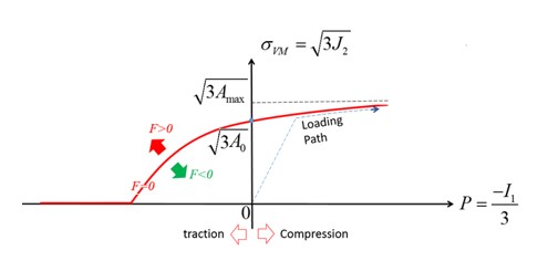
Рисунок 165: Критерии текучести Дрюкера-Прагера

Для описания давления \(A_{0}+A_{1}P+A_{2}P^{2}\) на поверхности текучести Дрюкера-Прагера материала используется полиномиальное уравнение: .. math:: sigma_{VM}=sqrt{3big{(}A_{0}+A_{1}P+A_{2}P^{2}big{)}} tag{128}

Константы полинома \(A_{0}, A_{1}, A_{2}\) определяются по формуле:

• Если \(F<0, J_{2}<A_{0}+A_{1}P+A_{2}P^{2}\) материал находится под поверхностью текучести и в упругой области.

• Если \(F=0, J_{2}=A_{0}+A_{1}P+A_{2}P^{2}\) и материал находится на поверхности текучести.

• Если \(F>0, J_{2}>A_{0}+A_{1}P+A_{2}P^{2}\) и материал вышел за пределы поверхности текучести и разрушился.

• Если \(A_{1}=A_{2}=0,\sigma_{VM}=\sqrt{3J_{2}}=\sqrt{3A_{0}}\), что является критерием фон Мизеса.

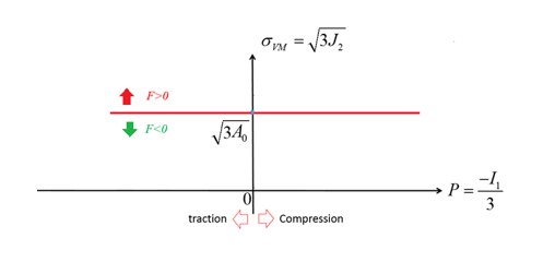
Рисунок 166:

Вычисление давления

В LAW10 для описания давления используется полиномиальное уравнение с входными параметрами \(C_{0}C_{1}C_{2}C_{3}\) . Давление можно построить как функцию объемной деформации.

\[\mu=\frac{\rho}{\rho_{0}}-1 \tag{129}\]

• Если \(P_{ext}=0\), давление равно \(P=\Delta P\), а предел давления равен \(P_{\min}=\Delta P_{\min}\).

width

4.72542in

height

2.30019in

Рисунок 167: Кривая давления без внешнего давления

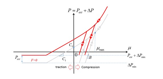
• Если \(P_{ext}\neq 0\), давление смещается на \(P_{ext}, тогда P=P_{ext}+\Delta P\) и предел давления равен \(P_{\min}=P_{ext}+\Delta P_{\min}\).

width

4.75042in

height

2.31686in

Рисунок 168: Кривая давления с внешним давлением

Здесь,

\[\begin{split}\Delta P=\left \{ \begin{matrix}\max\{\Delta P_{\min}\ C_{0}+C_{1}\mu+C_{2}\mu^{2}+C_{3}\mu^{3}\}if&\mu\geq 0compression \\ \max\{\Delta P_{\min}C_{0}+C_{1}\mu\}&if&\mu<0traction\end{matrix}\right|\end{split}\]

• При растяжении или натяжении давление линейно и ограничено \(\Delta P_{\min}\).

• При сжатии давление нелинейно и также ограничено \(\Delta P_{\min}\).

Единственное различие между материальными законами заключается в том, что в LAW10 материальные константы \(C_{0} C_{0} C_{2} C_{3}\) используются для описания давления в зависимости от объемной деформации (кривая \(P-\mu\)). В LAW21 вы можете описать эту кривую с помощью ввода функции fct_IDr.

Загрузка и разгрузка

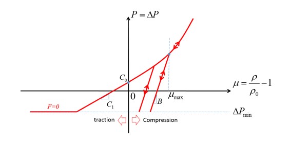
В LAW10 и LAW21 различные пути нагрузки и разгрузки кривой \(P-\mu\) можно рассматривать с использованием параметров \(\mu_{\max}\) и B.

• В напряжении (\(\mu<0)\)

  • Для LAW10 линейная загрузка и выгрузка с \(P=C_{1}\mu\) (рисунок 167).

  • Для LAW21 загрузка определяется с помощью входной функции fct_IDr и линейной разгрузки с помощью:math:P=K_{1}mu.

• В режиме сжатия \(\mu > 0\), for both LAW10 and LAW21:

  • Если не определены ни B, ни \(\mu_{\max}\), то пути загрузки и выгрузки идентичны.

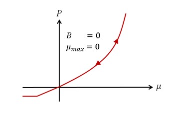
Рисунок 169: Идентичная загрузка и выгрузка для LAW10 и LAW21

• Если определено либо B, либо \(\mu_{\max}\):

1. Если определено только B, \(\mu_{\max}\) — это объемная деформация, где касательная к кривой \(P-\mu\) равна B с:math:B=frac{dP}{dmu}Big{|}_{mu_{max}}.

2. Если определено только \(\mu_{\max}\), то B является касательной к кривой \(P-\mu\) в \(\mu_{\max}\). Нагрузка и разгрузка при сжатии:

   • Если \(\mu>\mu_{\max}\), Путь загрузки и разгрузки идентичен.

   • Если \(\mu<\mu_{\max}\), Пути загрузки и разгрузки различны, это линейная разгрузка с уклоном B.

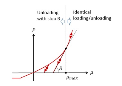
Рисунок 170: Различная обработка нагрузки и разгрузки для LAW10 и LAW21

Бетонный материал (/MAT/LAW24)

LAW24 использует критерии Дрюкера-Прагера с ограничением текучести или без него для моделирования армированного бетонного материала. Этот закон материала предполагает, что два механизма разрушения бетонного материала — это растрескивание при растяжении и сжатие.

Поведение бетона при растяжении

В LAW24 параметры \(H_{t}, D_{sup}\) и \(\varepsilon_{\max}\) могут использоваться для описания растрескивания при растяжении и разрушения при растяжении.

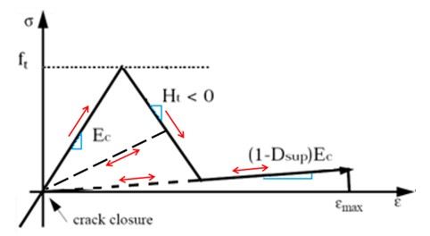
Рисунок 171: Растягивающая нагрузка LAW24

В начальной очень малой упругой фазе материал имеет модуль упругости \(E_{c}\).

После достижения предела прочности на растяжение \(f_{t}\) бетон начинает размягчаться с наклоном \(H_{t}\). Максимальный коэффициент повреждения \(D_{sup}\) имеет значение, поскольку он позволяет моделировать остаточную жесткость во время и после трещины.

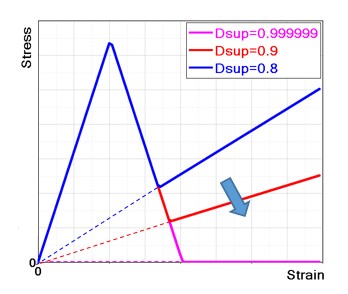
Рисунок 172: Максимальные эффекты фактора повреждения

Остаточная жесткость вычисляется как:

\[E=\left(1-D_{\text{sup}}\right)\cdot E_{c} \tag{131}\]

Когда происходит закрытие трещины, бетон снова становится эластичным, и фактор повреждения (для каждого направления) сохраняется.

Несущая способность бетона при растяжении намного ниже, чем при сжатии. Обычно он считается эластичным при растяжении.

Рекомендуется выбирать значение \(D_{sup}\) близкое к 1 (по умолчанию 0,99999), чтобы минимизировать текущую жесткость в конце повреждения и, следовательно, избежать остаточного напряжения при растяжении, которое может стать очень высоким, если элемент сильно деформирован из-за растяжения. Это произойдет, если сила, вызывающая повреждение, останется.

Можно настроить \(D_{sup} (и H_{t})\), чтобы смоделировать и подогнать поведение бетона, армированного волокнами. Бетонный материал разрушается, как только достигает полной деформации разрушения \(\varepsilon_{\max}\).

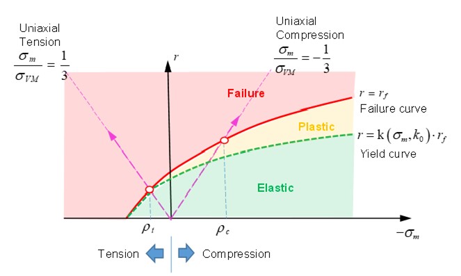
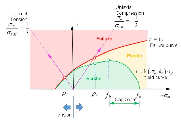
Поверхность текучести бетона при сжатии

Для бетона поверхность текучести является началом зоны пластического упрочнения, которая находится между поверхностью разрушения, \(r_{f}\), и поверхностью текучести.

Поверхность текучести предполагается такой же, как поверхность разрушения в зоне растяжения. При сжатии поверхность текучести представляет собой уменьшенную поверхность разрушения с использованием коэффициента k(\(\left(\sigma_{m},k_{0}\right))\). Выход в LAW24 для бетона:

\[f=\frac{r}{J_{2}}-\frac{\text{k}\left(\sigma_{m},k_{0}\right)\cdot r_{f}}{I_{part}}=0 \tag{132}\]

• Для \(I_{cap}\) =0 или 1 (без ограничения выхода) кривая выхода:

width

5.52549in

height

3.30863in

Рисунок 173: Критерии Дрюкера-Прагера без ограничения выхода

• Для \(I_{cap}\) =2 (с пределом текучести) выход равен:

width

5.24213in

height

3.52531in

Рисунок 174: Критерии Дрюкера-Прагера с пределом текучести

\(r<k\big{(}\sigma_{m},k_{0}\big{)}\cdot r_{f}\) (зеленая область на рисунке 174)

Материал находится под пределом текучести в упругой фазе.

\(r\geq r_{f}\) (красная область на рисунке 174)

Материал не выдержал испытания.

\(k\big{(}\sigma_{m},k_{0}\big{)}\cdot r_{f}<r<r_{f}\) (желтая область на рисунке 174)

Материал находится выше предела текучести и ниже поверхности разрушения, которая представляет собой фазу пластического упрочнения.

Входной параметр \(\rho_{t}\) — это гидростатическое давление разрушения при одноосном испытании на растяжение, а \(\rho_{c}\) — это гидростатическое давление при разрушении при одноосном испытании на сжатие.

Масштабный коэффициент \(k\big{(}\sigma_{m},k_{0}\big{)}\) является функцией среднего напряжения \(\sigma_{m}\) и может быть описан как:

• Когда

  \(\sigma_{m}\geq\rho_{t}\) (при растяжении) масштабный коэффициент \(k\big{(}\sigma_{m},k_{0}\big{)}=1)\). В этом случае поверхность текучести равна поверхности разрушения, \(r=r_{f}\).

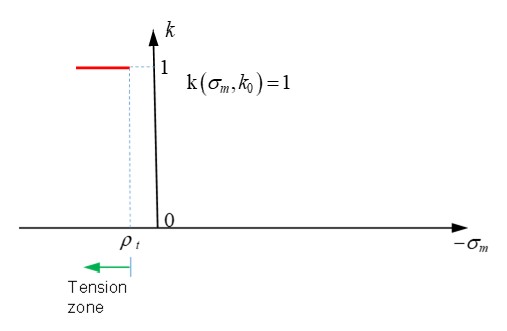
Рисунок 175: k-функция в зоне растяжения

• В области растяжения-сжатия, \(\rho_{t}>\sigma_{m}\geq\rho_{c,}\) затем

\(\mathrm{k}\big{(}\sigma_{m} k_{0}\big{)}=1+\frac{\big{(}1-k_{0}\big{)}\cdot\Big{[}\rho_{t}\big{(}2\rho_{c}-\rho_{t}\big{)}-2\rho_{c}\sigma_{m}+\sigma_{m}\Big{]}}{\big{(}\rho_{c}-\rho_{t}\big{)}^{2}} \mathrm{with} k_{y}\leq k_{0}\leq 1\)

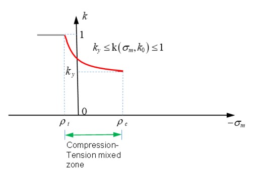
Рисунок 176: функция k в зоне сжатия-растяжения

• Остальная часть кривой зависит от опции \(I_{cap}\) и различных используемых масштабных коэффициентов \(k\big{(}\sigma_{m},k_{0}\big{)}\).

  ◦ Для \(I_{cap}\) =0 or 1 and \(\sigma_{m}<\rho_{c}\) (при сжатии), то \(k\big{(}\sigma_{m},k_{0}\big{)}=k_{y}\)

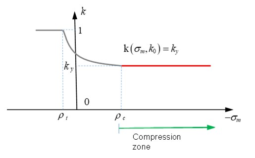
Рисунок 177: Функция K в зоне сжатия

◦ Для \(I_{cap}\) =2 (с пределом доходности) и \(\rho_{c}<\sigma_{m}<f_{k}\) (при сжатии), то \(k\big{(}\sigma_{m},k_{0}\big{)}=k_{y}\)

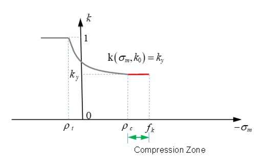
Рисунок 178: Функция K в критериях Дрюкера-Прагера без ограничения

◦ В \(f_{k}<\sigma_{m}<f_{0}\) (в кеп-зоне)

\(\mathrm{k}\big{(}\sigma_{m},k_{0}\big{)}=k_{0}\bigg{[}1-\bigg{(}\frac{\sigma_{m}-f_{k}}{f_{0}-f_{k}}\bigg{)}^{2}\bigg{]},\mathrm{with} 0\leq k_{0}\leq k_{y}\)

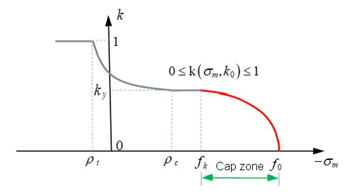
Рисунок 179: Функция K в критериях Дрюкера-Прагера без ограничения

Константа материала \(k_{y}\) должна быть \(0\leq k_{y}\leq 1\). Более высокое значение \(k_{y}\) приводит к более высокой поверхности текучести. Например, если \(I_{cap}=2\) (текучесть с ограничением), разница в поверхности текучести между \(k_{y}=0,8\) и \(k_{y}=0,6\) (Рисунок 180). Значение по умолчанию \(k_{y}\) в LAW24 равно 0,5.

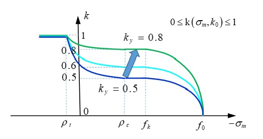
Рисунок 180: После различных значений функции K

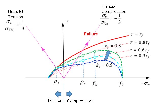
Рисунок 181: Критерии Дрюкера-Прагера с различными значениями функции K

Правило пластического течения бетона при сжатии

В LAW24 используется неассоциированное правило пластического течения. Правило пластического течения:

\[g=\alpha I_{1}+\sqrt{J_{2}} \tag{133}\]

Где,

\(\alpha\) Пластическая дилатансия.

\(\alpha=\frac{\partial g}{\partial I_{1}}\) Управляет объемным пластическим течением.

\(I_{1}\) Первый инвариант напряжения (гидростатическое давление).

Экспериментально \(\alpha\) является линейной функцией \(k_{0}\):

\[\alpha=\frac{\big{(}1-k_{0}\big{)}\alpha_{y}+\big{(}k_{0}-K_{y}\big{)}\alpha_{f}}{1-K_{y}} \tag{134}\]

Если\(k_{0}=K_{y}\) то, \(\alpha=\alpha_{y}\) что означает, что материал находится в состоянии текучести.

Если\(k_{0}<K_{y}\) тогда, \(\alpha\) становится отрицательным, это область крышки.

Если\(k_{0}=1\) тогда, \(\alpha=\alpha_{f}\) что означает, что материал разрушился. Значения \(\alpha_{y}, \alpha_{f}\) используются для описания материала за пределами текучести, но до разрушения. Рекомендуется использовать -0,2 и -0,1 для \(\alpha_{y}, \alpha_{f}\) в LAW24. Если используются очень малые значения \(\alpha_{y}, \alpha_{f}\), то объемная пластичность отсутствует (область крышки отсутствует).

Разрушение бетона при сжатии

Поверхность разрушения определяется по формуле:

\[f=r-r\_{f}(\sigma_{mp} \theta)=0 \tag{135}\]

Где, \(r=\sqrt{2J_{2}}\left/\int_{c}\sigma_{m}=I_{1}\right/3f_{c}\). и \(\тета\) — угол Лоде, например:

\[\mathrm{cos}3\theta=\frac{J_{3}}{2}\bigg{(}\frac{3}{J_{2}}\bigg{)}^{3/2} \tag{136}\]

Поверхность Оттозена строится для проектирования этой поверхности с использованием:

\[r_{f}(\sigma_{m} \theta)=\frac{1}{a}\Big{(}-b+\sqrt{b^{2}-a(\sigma_{m}-c)} \Big{)} \tag{137}\]

Где, \(a, b_{c}, b_{i} и c\) — это 4 значения, которые формируют поверхность и

\[b(b_{c}, b_{p}, \theta)=\frac{1}{2}\Big{[}b_{c}(1-\mathrm{cos}3\theta)+b_{1}(1+\mathrm{cos}3\theta)\Big{]} \tag{138}\]

Для бетона сжатие Кривая разрушения \(r_{f}\) может быть определена с прочностью:

\(f_{t}\) Одноосное растяжение (триаксиальность составляет 1/3)

\(f_{c}\) Одноосное сжатие (триаксиальность составляет -1/3)

\(f_{b}\) Двуосное сжатие (триаксиальность составляет -2/3)

\(f_{2}\) Прочность на ограниченное сжатие (трехосное испытание)

\(s_{0}\) Под ограниченным давлением Лучший способ полностью определить трехмерную область разрушения — получить экспериментальные данные для всех этих значений, \(f_{c} f_{f} f_{b} f_{2} s_{0}\), которые схематически проиллюстрированы на рисунке 182. .. image:: vertopal_75794439f47d439ba01f734ac3f4dcc1/media/image5-3.jpg

width

5.80883in

height

3.55031in

Рисунок 182: Параметры отказа, которые полностью определяют трехмерную огибающую отказа

Рисунок 183 и Рисунок 184 показывают точки, которые определяют поверхность отказа.

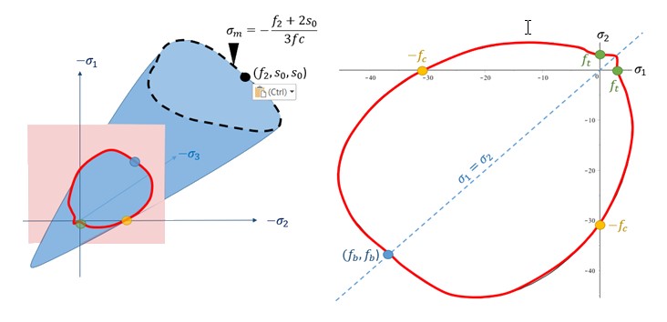
Рисунок 183: След поверхности разрушения с плоской плоскостью напряжения .. image:: vertopal_75794439f47d439ba01f734ac3f4dcc1/media/i-mage55.jpg

width

6.09219in

height

2.9836in

Рисунок 184: Траектория разрушения с несколькими планами разреза, которые перпендикулярны гидростатической оси

Из этих графиков следует, что область разрушения не является выпуклой поверхностью. Рисунок 185 показывает это поведение.

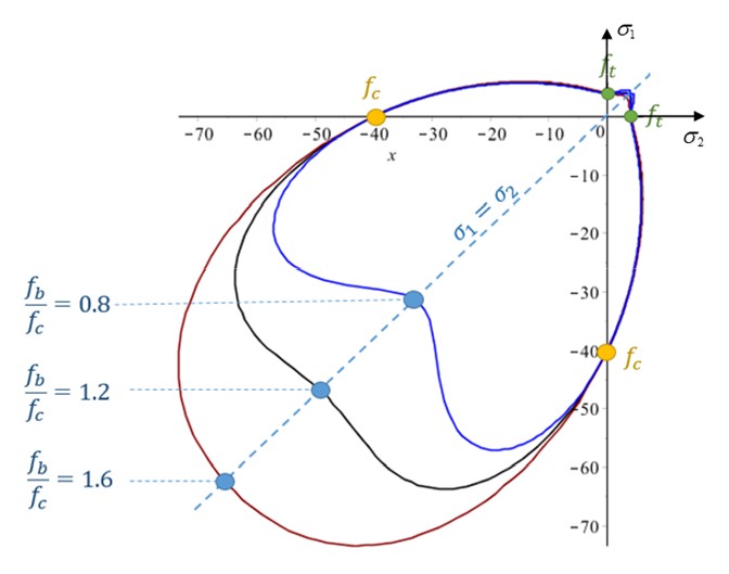
Рисунок 185: Влияние значения прочности на двухосное сжатие при всех других фиксированных характерных точках разрушения .. image:: vertopal_75794439f47d439ba01f734ac3f4dcc1/media/image5-7.jpg

width

4.95043in

height

4.80042in

Рисунок 186: Влияние значения прочности на сжатие при всех других фиксированных характерных точках разрушения

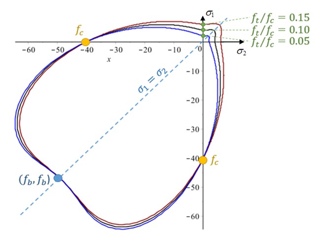
Рисунок 187: Влияние значения прочности на растяжение при всех других фиксированных характерных точках разрушения

В этом конкретном случае прочность на сжатие меняется, но все остальные соотношения фиксированы

. Это приводит к масштабированию огибающей, как показано на рисунке 188.

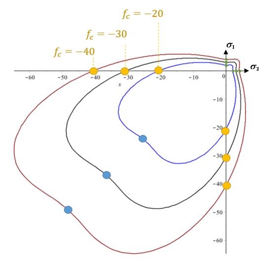
Рисунок 188: Влияние значения прочности на сжатие

Все остальные соотношения фиксированы.

Здесь с той же прочностью в LAW24, но с другой прочностью на ограниченное сжатие \(f_{2}\)

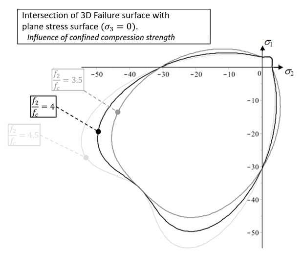
Рисунок 189: Огибающая разрушения на поверхности плоского напряжения, на которую влияет точка трехосного разрушения

\(\left(\sigma_{1,}\sigma_{2,}\sigma_{3}\right)=\left(f_{2,}s_{0,}s_{0}\right)\)

\(f_{c}\) и соотношения \(f_{t}/f_{c}\) и \(f_{b}/f_{c}\) in the :math:`r-sigma_{m} пространство (используемое для определения разрушения бетона):

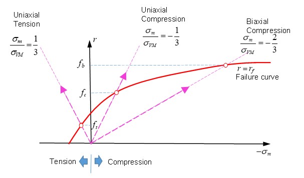
Рисунок 190: Различные испытания (одноосное растяжение, одноосное сжатие и двухосное сжатие) для определения кривой разрушения

Если кривая разрушения определяется с помощью \(r=\sqrt{2J_{2}}=\sqrt{\frac{2}{3}} \sigma_{YM}\) и \(\sigma_{m}=\frac{I_{1}}{3}\) — среднее напряжение (давление), то \(I_{1}\) и \(J_{2}\) — первый и второй инварианты напряжения.

Материал разрушается, как только достигает кривой разрушения \(r_{f}\).

Армирование бетона

В PRADIOS есть два разных способа моделирования арматуры в бетоне.

• Один способ - использовать балочные или ферменные элементы и соединить их с бетоном с помощью кинематических условий.

• Другой способ - использовать параметры в LAW24 вместе с ортотропным свойством твердого тела /PROP/ TYPE6 для определения направления армирования. Параметры \(a_{1}, a_{2}, a_{3}\) в LAW24 используются для определения отношения площади поперечного сечения арматуры ко всей площади сечения бетона в направлении 1, 2, 3.

\[a_{i}=\frac{Area_{steel}}{Area_{concrete}} \tag{138}\]

Где, \(\sigma_{y}\) - предел текучести арматуры. Если в качестве арматуры используется сталь, то \(\sigma_{y}\) — предел текучести стали, а \(E_{t}\) — модуль упругости стали в пластической фазе. .. image:: vertopal_75794439f47d439ba01f734ac3f4dcc1/media/image6-2.jpg

width

3.30863in

height

2.14185in

Рисунок 191: Кривая напряжения-деформации арматуры (сталь)

Бетонный материал (/MAT/LAW81)

LAW81 можно использовать для моделирования материалов из камня или бетона.

Критерии текучести Дрюкера-Прагера

LAW81 использует критерий текучести Дрюкера-Прагера, где поверхность текучести и поверхность разрушения одинаковы. Критерий текучести: .. math:: F=frac{q}{J_{2},text{part}}-frac{text{r}_{c}(p)cdotbig{(}text{ptan}phi+cbig{)}}{I_{1},text{part}}=0 tag{140}

Где,

\(q\) Стресс фон Мизеса с \(q=\sigma_{VM}=\sqrt{3J_{2}}\)

\(p\) Давление определяется как \(p=\frac{1}{3}I_{1}\)

12. Han, D. J., и Вай-Фа Чен. “Модель пластичности неравномерного упрочнения для бетонных материалов.” Механика материалов 4, no. 3-4 (1985): 283-302

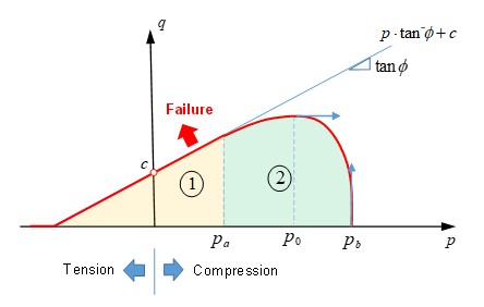
Рисунок 192: Поверхность текучести (LAW81)

Поверхность текучести можно описать двумя частями:

• Линейная часть (\(p\leq p_{a})\), где масштабная функция равна \(\mathrm{r}_{c}(p)=1\), что приводит к тому, что напряжение по Мизесу линейно пропорционально давлению:

\[q=p\mathrm{tan}\phi +c \tag{141}\]

Где,

\(c\) Когезионный и является точкой пересечения огибающей текучести с пределом прочности на сдвиг.

Если \(c\) =0, материал не имеет прочности при растяжении.

\(\phi\) Угол внутреннего трения, который определяет наклон огибающей текучести.

\(c\) и \(\phi\) также используются для определения поверхности текучести Мора-Кулона. Поверхность текучести Дрюкера-Праге является гладкой версией поверхности текучести Мора-Кулона.

• Вторая часть (\(p_{a}<p<p_{b})\) поверхности текучести имитирует предел текучести. Увеличение давления в камне или бетонном материале увеличит текучесть материала; но если давление увеличится достаточно, то камень или бетонный материал будет раздавлен. Модель Дрюкера-Прагера с пределом текучести может быть использована для моделирования этого поведения. Предел текучести определен в части и использует функцию масштабирования:

\[\mathrm{r}_{c}\big{(}p\big{)}=\sqrt{1-\left(\frac{p-p_{a}}{p_{b}-p_{a}}\right)^{2}} \tag{142}\]

Напряжение фон Мизеса равно:

\[q=\sqrt{1-\left(\frac{p-p_{a}}{P_{b}-\overline{p}_{a}}\right)^{2}}\cdot\left(p\text{tan}\phi+c\right) \tag{143}\]

Где,

\(P_{b}\) Кривая определяется с использованием входных данных \(fct_ID_{Pb}\)

\(p_{a}\) Рассчитано PRADIOS с использованием входного значения отношения \(a\).

\(p_{a}=\alpha\cdot P_{b}\) с \(0<\alpha <1\).

Где, \(P_{0}\) — максимальная точка кривой текучести, где \(\frac{\partial F}{\partial p}\left(p_{0}\right)=0\)

Если \(p=p_{b}\), то \(r_{\text{c}}\left(p_{b}\right)=0\) и функция текучести тогда,

\(q=0:\cdot\left(p\text{tan}\phi+c\right)=0\) что означает, что материал раздроблен.

Входные параметры \(\phi, c, p_{b^{\prime}}\alpha\) необходимо определить для поверхности текучести Друкера-Прагера. Для соответствия этим параметрам необходимо провести не менее четырех испытаний. В простейшем случае одноосное растяжение и одноосное сжатие можно использовать для определения линейной части, \(\phi, \text{и} c\). Для определения \(p_{b^{\prime}\) и \(\alpha\) необходимы двухосные испытания на сжатие и испытания на сжатие/сжатие (см. CC00 и CC01 в RD-E: 4701 Проверка бетона с помощью испытаний Купфера).

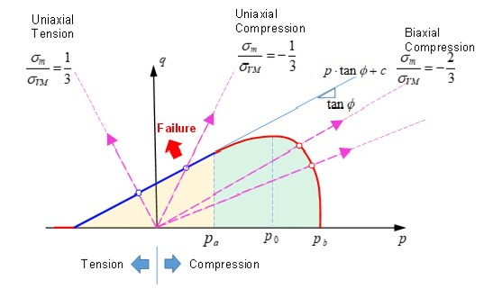
Рисунок 193: Поверхность текучести LAW81, показывающая различные условия нагрузки

Для большинства материалов, таких как металл, приращение пластической деформации можно считать нормальным к поверхности текучести. Однако, если приращение пластической деформации нормально к поверхности текучести используется для материалов из камня или бетона, расширение пластического объема переоценивается. Поэтому в этих материалах используется неассоциированное правило пластического течения. В LAW81 функция пластического течения G определяется как:

• \(G=q-p\cdot\tan\psi=0 if p\leq p_{a}\)

• \(G=q-\tan\psi\left(p-\frac{\left(p-p_{a}\right)^{2}}{2\left(p_{0}-p_{a}\right)}\right)=0 if p_{a}<p\leq p_{0}\)

• \(G=F if p>p_{0}\)

Поскольку давление равно \(p_{0}\), то функция текучести F и функция пластического течения G одинаковы и выполняется следующее условие:

\[G(p_{0})=F(p_{0}) \tag{144}\]

\[\frac{\partial G}{\partial p}|{p_{0}}=\frac{\partial F}{\partial p}|{p_{0}}=0 \tag{145}\]

Давление \(p\_{0}\) можно рассчитать с помощью поверхности текучести, где \(\frac{\partial F}{\partial p}| p_{0}=0\). Если G определено как:

\[G=q-\tan\psi\left(p-\frac{\left(p-p_{a}\right)^{2}}{2\!\left(p_{0}-p_{a}\right)}\right)=0 \tag{146}\]

Параметр \(\psi\) можно определить, используя напряжение фон Мизеса при давлении, \(p_{0}\) в функции.

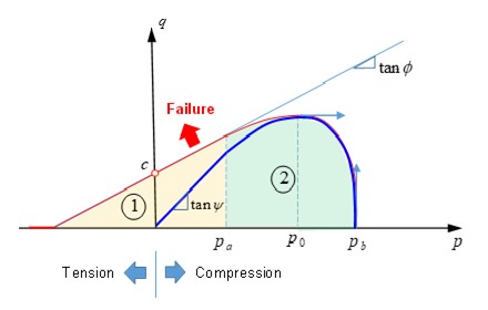
Рисунок 194: Поверхность текучести LAW81 с пластическим течением

Разрушение

Пластичное

Модели разрушения /FAIL/BIQUAD, /FAIL/JOHNSON и /FAIL/TAB1 определяют разрушение материала, связывая пластическую деформацию при разрушении с напряженным состоянием в материале.

Эти модели разрушения часто используются для описания пластичного разрушения материалов. Состояние напряжения в материале можно определить с помощью триаксиальности напряжения.

Триаксиальность напряжения (нормализованное среднее напряжение)

Для пластичных материалов состояние напряжения (сжатие, сдвиг, растяжение и т. д.) материала влияет на значение пластической деформации, при которой материал разрушится. Важная и полезная характеристика для описания состояния напряжения, трехосность напряжения определяется как:

\[\sigma^{*}=\frac{\sigma_{m}}{\sigma_{VM}} \tag{147}\]

Где,

:math:`sigma_{m}=frac{1}{3}big{(}sigma_{1}+sigma_{2}+sigma_{3}big{)}`Среднее (гидростатическое) напряжение

\(\sigma_{VM}=\sqrt{\frac{1}{2}\big{[}\big{(}\sigma_{1}-\sigma_{2}\big{)}^{2}+\big{(}\sigma_{2}-\sigma_{3}\big{)}^{2}+\big{(}\sigma_{3}-\sigma_{1}\big{)}^{2}\big{]}}\) Мизес стресс

Значения трехосности для некоторых состояний общего напряжения можно получить следующим образом:

• При чистом растяжении:

  \(\sigma_{2}=\sigma_{3}=0\) then \(\sigma^{*}=\frac{\sigma_{m}}{\sigma_{VM}}=\frac{1}{3}\)

• При двухосном сжатии:

  \(\sigma_{1}=\sigma_{2}\), и \(\sigma_{3}=0\), тогда \(\sigma^{*}=\frac{\sigma_{m}}{\sigma_{VM}}=-\frac{2}{3}\)

Трехосность напряжения для различных напряженных состояний:

Трехосность напряжения \(\sigma^{*}\) Напряженное состояние

\(-\frac{2}{3}\) Двуосное сжатие

\(-\frac{1}{3}\) Одноосное сжатие

\(\textbf{0}\) Чистый сдвиг

\(\frac{1}{3}\) Одноосное растяжение

\(\frac{1}{\sqrt 3}\) Плоская деформация

\(\frac{2}{3}\) Двуосное растяжение

/FAIL/JOHNSON

Модель разрушения Джонсона-Кука часто используется для описания пластичного разрушения металлов. Она использует уравнение Джонсона-Кука для определения деформации разрушения как функции трехосности напряжения.

В модели неудач Джонсона-Кука есть три части;

\[\varepsilon_{f}=\big{[}D_{1}+D_{2} exp(D_{3}\sigma^{*})\big{]}\big{[}1+D_{4}in(\varepsilon^{*})\big{]}\big{[}1+D_{5}T^{*}\big{]} \tag{148}\]

Где

\(\varepsilon_{f}\) Пластическая деформация разрушения

\(\varepsilon^{*}=\frac{\varepsilon}{\varepsilon_{0}}\) Текущая скорость деформации, деленная на входную опорную скорость деформации

\(T^{*}\) Рассчитано по материальному закону или /HEAT/MAT

Игнорируя влияние скорости деформации и температуры, график разрушения Джонсона-Кука выглядит следующим образом:

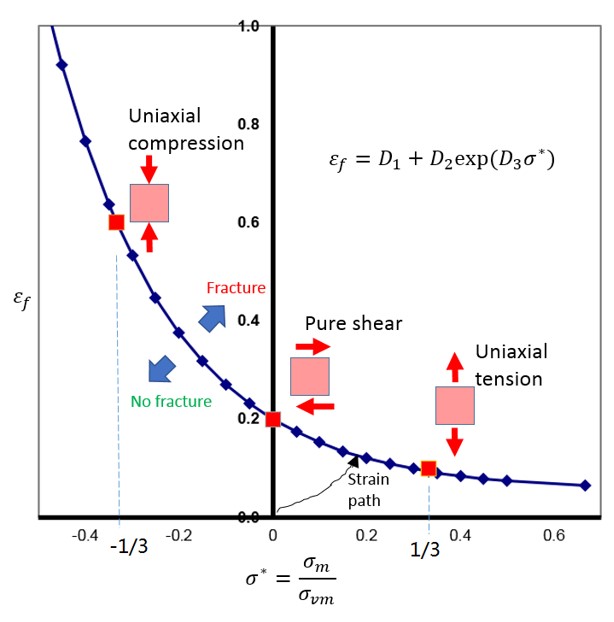
Рисунок 195: Пример графика модели разрушения Джонсона-Кука

Пластические деформации над кривой представляют собой разрушение материала, а под кривой — отсутствие разрушения материала.

В простом случае, когда учитывается только влияние трехосности, деформация разрушения равна:

\[\varepsilon_{f}=\mathrm{D}_{1}+\mathrm{D}_{2}\cdot\exp\bigl{(}\mathrm{D}_{3}\cdot\sigma^{\bullet}\bigr{)} \tag{149}\]

Используя 3 точки данных разрушения из теста:

\(\varepsilon_{f}=0,1585\) при одноосном растяжении (\(\sigma^{\bullet}=1/3)\)

\(\varepsilon_{f}=0,19\) при чистом сдвиге (\(\sigma^{\bullet}=0)\)

\(\varepsilon_{f}=0,2419\) при одноосном сжатии (\(\sigma^{\bullet}=-1/3)1\)

Параметры \(\mathrm{D}_{1}, :math:\)mathrm{D}_{2}` и \(\mathrm{D}_{3}\) можно вычислить аналитически, решив следующие уравнения:

\[\tag{150}\]

\[\begin{split}\left \{ \begin{matrix} 0.1585=\mathrm{D}_{1}+\mathrm{D}_{2}\cdot\exp\bigl{(}\mathrm{D}_{3}\cdot \tfrac{1}{3}\bigr{)} \\ 0.19=\mathrm{D}_{1}+\mathrm{D}_{2}\cdot\exp\bigl{(}\mathrm{D}_{3}\cdot 0\bigr{)} \\ 0.2419=\mathrm{D}_{1}+\mathrm{D}_{2}\cdot\exp\bigl{(}\mathrm{D}_{3}\cdot-\tfrac{1}{3}\bigr{)}\end{matrix}\right|\end{split}\]

Обработка отказа элемента

Метод накопленного повреждения используется для суммирования величины пластической деформации, которая произошла в элементе, с использованием:

\[D=\sum\frac{\Delta\varepsilon_{p}}{\varepsilon_{f}}\geq 1\tag{151}\]

Что происходит, когда \(D\geq 1\) зависит от значений флагов отказа элемента (\(I_{fail_sh} и I_{fail_so})\) и флага формулировки XFEM (\(I_{\textit{xfem}})\). Когда формулировка XFEM не используется (\(I_{\textit{xfem}})=0\), следующая таблица суммирует различные варианты флага отказа элемента:

Таблица 18: Вариант отказа элемента

Элемент	Отказ элемента флаг	Если \(D\geq 1\)	Поведение при отказе
Shell	\(I_{fail_sh}\) =1 (Default)	в 1 IP или слой	Элемент удален.
Shell	\(I_{fail_sh}\) =2	в 1 IP или слой	тензор напряжения 0 im IP или слой
Shell	\(I_{fail_sh}\) =2	Все IP или слои	Элемент удален.
Solid	\(I_{fail_sh}\) =1 (по умолчанию)	в 1 IP	Элемент удален.
Solid	\(I_{fail_sh}\) =2	в 1 IP	тензор напряжения устан-н на 0 im IP
Solid	\(I_{fail_sh}\) =2	все IP	тензор напряжения уст-н 0 в элементы

Подробную информацию о формулировке XFEM (\(I_{\textit{xfem}})=1)\), можно найти в /FAIL/JOHNSON.

Повреждение, D, можно отобразить в файлах анимации с помощью /ANIM/SHELL/DAMA или /ANIM/BRICK/DAMA. Это покажет риск материального повреждения.

/FAIL/BIQUAD

В PRADIOS /FAIL/BIQUAD является наиболее удобной для пользователя моделью разрушения для пластичных материалов. Она использует упрощенные, нелинейные критерии разрушения на основе деформации с линейным накоплением повреждений.

Разрушение описывается двумя параболическими функциями, рассчитанными с использованием подгонки кривой из до 5 введенных пользователем деформаций разрушения.

По умолчанию /FAIL/BIQUAD (``S-Flag``=1) использует две параболические кривые для описания пластической деформации разрушения \(\varepsilon_{f}\), как функции трехосности напряжения \(\sigma\). Две параболические кривые используют:

\[f_{2}(x)=dx^{2}+ex+f \tag{152}\]

Где,

\(a, b, c, d, e,\) и \(f\) Параболические коэффициенты

\(x\) Трехосность напряжения

\(f_{1}(x)\) и \(f_{2}(x)\) Пластическая деформация разрушения

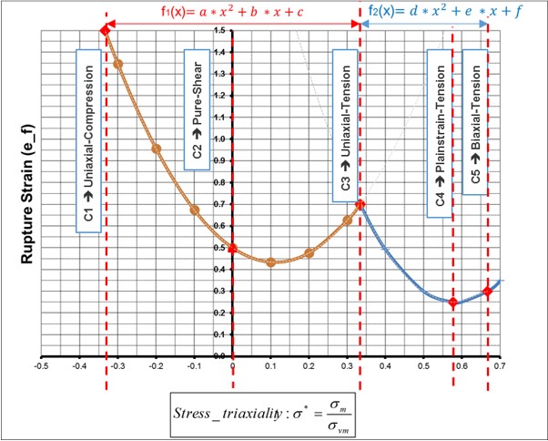
Рисунок 196: /FAIL/BIQUAD Кривая деформации разрушения, состоящая из 2 параболических

Параболические коэффициенты \(a, b, c, d, e,\) и \(f\) вычисляются PRADIOS с использованием подгонки кривой на основе входных значений пластической деформации разрушения c1-c5. Если рассчитанные параболические кривые деформации разрушения имеют отрицательные значения деформации разрушения, эти отрицательные значения будут заменены на деформацию разрушения 1E-6, что приводит к очень высокому накоплению повреждений и хрупкому поведению. Результаты подгонки кривой находятся в файле Starter *0000.out.

   Би-квадратичный ОТКАЗ
     - - - - - - - - - - - - - -
c1. . . . . . . . . . . . . . . . . . .= 0.2419E+00
c2. . . . . . . . . . . . . . . . . . .= 0.1900E+00
c3. . . . . . . . . . . . . . . . . . .= 0.1585E+00
c4. . . . . . . . . . . . . . . . . . .= 0.1437E+00
c5. . . . . . . . . . . . . . . . . . .= 0.1394E+00
   КОЭФФИЦИЕНТЫ ПЕРВОЙ ПАРАБОЛЫ
     - - - - - - - - - - - - - -
a . . . . . . . . . . . . . . . . . . .= 0.9180E-01
b . . . . . . . . . . . . . . . . . . .= -0.1251E+00
c . . . . . . . . . . . . . . . . . . .= 0.1900E+00
   КОЭФФИЦИЕНТЫ ВТОРОЙ ПАРАБОЛЫ
     - - - - - - - - - - - - - -
d . . . . . . . . . . . . . . . . . . .= 0.3753E-01
e . . . . . . . . . . . . . . . . . . .= -0.9483E-01
f . . . . . . . . . . . . . . . . . . .= 0.1859E+00

Определения пластических деформаций разрушения c1–c5 следующие:

c1

Пластическая деформация разрушения при одноосном сжатии

c2

Пластическая деформация разрушения при сдвиге

c3

Пластическая деформация разрушения при одноосном растяжении

c4

Пластическая деформация разрушения при плоском растяжении

c5

Пластическая деформация разрушения при двухосном растяжении

Параметры ввода M-Flag

В зависимости от параметра ввода M-Flag существует три различных способа определения значений c1-c5.

1001. • M-Flag=0, Пользовательские данные испытаний В этом случае необходимо ввести c1-c5, что представляет собой пластическую деформацию разрушения для 5 различных напряженных состояний. В идеале эти данные следует получить из испытаний или от поставщика материалов.

1002. • M-Flag=1-7, Предопределенные данные материалов Если данные о деформации разрушения недоступны, можно выбрать из 7 предопределенных материалов. На рисунке 197 показаны кривые пластической деформации при разрушении для 7 материалов.

Примечание: Предопределенные значения предоставляются для раннего исследования конструкции, и вы несете ответственность за проверку того, что их материал имеет те же свойства… image:: vertopal_75794439f47d439ba01f734ac3f4dcc1/media/image72.png

width

4.60333in

height

3.36667in

Рисунок 197: Предопределенные кривые разрушения материала

• M-Flag=99, Ввод коэффициента деформации пластического разрушения, r1-r5

Последний метод ввода — ввести пластическую деформацию разрушения при одноосном растяжении, c3, и коэффициенты пластической деформации разрушения для остальных четырех напряженных состояний. Эти коэффициенты определяются как:

r1

Отношение пластической деформации разрушения, одноосное сжатие (c1) к одноосному растяжению (c3), поэтому \(c1=r1\cdot c3\)

r2

Отношение пластической деформации разрушения, чистый сдвиг (c2) к одноосному растяжению (c3), поэтому \(c2=r2\cdot c3\)

r4

Отношение пластической деформации разрушения, плоское растяжение (c4) к одноосному растяжению (c3), поэтому \(c4=r4\cdot c3\)

r5

Отношение пластической деформации разрушения, двуосное растяжение (c5) к одноосному растяжению (c3), поэтому \(c5=r5\cdot c3\)

Используя этот метод, можно легко изменить кривую разрушения, регулируя единичную пластическую деформацию разрушения при одноосном растяжении, c3.

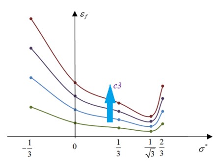
Рисунок 198: Изменения в кривой пластической деформации разрушения путем увеличения одноосного разрушения растяжением, c3, с теми же коэффициентами пластической деформации разрушения

Поведение по умолчанию

По умолчанию для c1 по c5 необходимо ввести значения, отличные от 0. Однако существуют определенные поведения по умолчанию, в случае отсутствия информации об отказе.

• Если поведение разрушения материала неизвестно, c1 по c5 устанавливаются на 0,0, и используется поведение мягкой стали (M-Flag=1).

• Если известно только значение разрушения при растяжении, определяется c3 (c1=c2=c4=c5=0,0). Поведение мягкой стали используется и масштабируется с помощью определенного пользователем значения c3.

• В случае, если поведение материала известно, M-Flag определяется, и c3 может использоваться для корректировки модели отказа в соответствии с ожидаемым разрывом при растяжении. Выбранное поведение материала масштабируется с помощью определенного пользователем значения c3.

• Для всех остальных случаев все c1 - c5 должны быть определены, и используется значение по умолчанию 0,0.

Обработка отказа элемента

Метод накопленного повреждения используется для суммирования величины пластической деформации, которая произошла в каждой точке интегрирования в элементе, используя:

\[D=\sum\frac{\Delta\varepsilon_{p}}{\varepsilon_{f}}\geq 1 \tag{154}\]

Где,

D Повреждение

\(\Delta\varepsilon_{p}\) Изменение пластической деформации точки интегрирования

\(\varepsilon_{f}\) Пластическая деформация разрушения для текущего напряжения триаксиальности

В оболочечных элементах после того, как точка интегрирования достигает D*=1, тензор напряжений точки интегрирования устанавливается равным нулю. Элемент выходит из строя и удаляется, когда отношение точек интегрирования по толщине, не прошедших проверку, равняется *P_thickfail. В объемных элементах элемент удаляется, когда любая точка интегрирования достигает .

Плоская деформация как глобальный минимум

Опция S-Flag=2 может использоваться для принудительного достижения глобального минимума кривой пластической деформации разрушения в месте напряжения плоской деформации триаксиальности, c4. Это достигается путем разделения второго уравнения на 2 отдельные квадратичные подфункции.

Моделирование нестабильности материала (локальное сужение)

В таких материалах, как листовой металл, истончение толщины и диффузное утолщение могут появляться во время растягивающей нагрузки материала. Это называется локализованным утолщением и обычно происходит в диапазоне напряжений триаксиальности \(\frac{1}{3}\leq\sigma^{\bullet}\leq\frac{2}{3}:\)

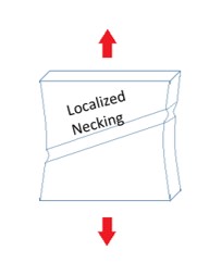
Рисунок 199:

В /FAIL/BIQUAD можно смоделировать это локализованное сужение, используя опцию S-Flag=3 и Inst_start. Эта опция использует ту же кривую пластической деформации разрушения, что и S-Flag=2, и добавляет две дополнительные квадратичные функции, которые определяют кривую, которая представляет начало локализованного сужения между трехосностью напряжения \(\frac{1}{3}\) и \(\frac{2}{3}\). Минимальное значение этой кривой задается пользователем в поле Inst_start и возникает при плоской деформации растяжения \(\sigma^{*}=\frac{1}{\sqrt{3}}\). Используя эту локализованную кривую сужения, вычисляется второе значение повреждения локализованного сужения, и отказ из-за сужения происходит только тогда, когда все точки интегрирования достигают \(D=\mathrm{I}\). Критерий локализованного сужения основан на анализе Марциняка-Кучински.¹³ .. image:: vertopal_75794439f47d439ba01f734ac3f4dcc1/media/im-age75.jpg

width

3.59197in

height

2.85025in

Рисунок 200: Кривая деформации разрушения по умолчанию с дополнительной кривой локализованного образования шейки (синяя)

При использовании S-Flag=1 или 2 накопление повреждений начинается, как только пластическая деформация достигает кривой разрушения (красная на рисунке 201).

Если S-Flag=3 используется для описания локализованного образования шейки, накопление повреждений начинается, как только пластическая деформация достигает кривой локализованного образования шейки (синяя кривая на рисунке 201). Для локализованного образования шейки элемент удаляется, когда все точки интегрирования достигают повреждения, D*=1, тогда как удаление элемента не из-за локализованного образования шейки определяется *P_thickfail. *Risunok 200: Krivaya deformatsii

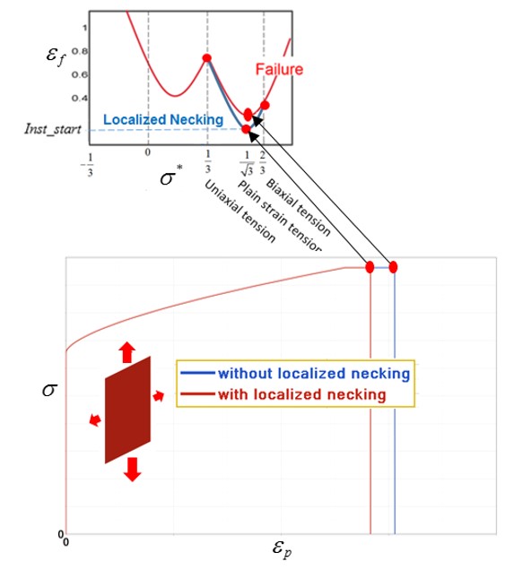
Рисунок 201:

Возмущение предела разрушения

Из-за несовершенства материалов или производственного процесса деформация разрушения материала может быть не везде одинаковой, и, таким образом, могут существовать очень небольшие возмущения предела разрушения. При использовании M-Flag>0 с /PERTURB/FAIL/BIQUAD статистическое распределение предела разрушения применяется к каждому элементу, которому назначена модель разрушения. Это достигается путем вычисления нормального или случайного распределения масштабного коэффициента разрушения, который применяется к /FAIL/BIQUAD, c3. Два различных метода распределения показаны на рисунке 202 и рисунке 203.

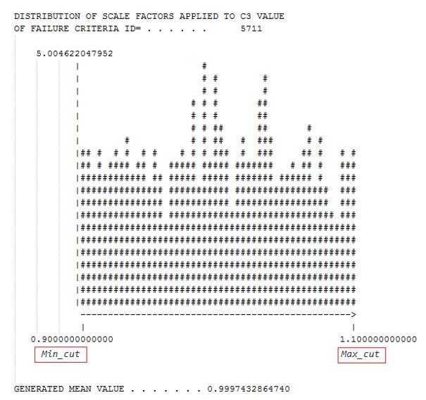
Рисунок 202: Случайное распределение Idistri=1, предела отказа в файле Starter 0.out

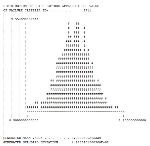
Рисунок 203: Нормальное (гауссовское) распределение Idistri=2 предела отказа в файле Starter *0.out **

/FAIL/BQUAD использует небольшие возмущения c3, созданные /PERTURB/FAIL/BIQUAD для масштабирования всей кривой отказа с использованием значений коэффициента деформации для предопределенных материалов или определяемых пользователем коэффициентов, r1, r2, r4 и r5, в зависимости от значения M-Flag. .. image:: vertopal_75794439f47d439ba01f734ac3f4dcc1/media/imuge104.jpg

width

4.9921in

height

4.00035in

Рисунок 204:

Ссылка

Табличная модель отказа /FAIL/TAB1

В PRADIOS /FAIL/TAB1 является самой сложной моделью отказа для пластичного материала. Пластическая деформация отказа может быть определена как функция: трехосности напряжения, скорости деформации, угла Лоде, размера элемента, температуры и деформации нестабильности.

Повреждение накапливается на основе определяемых пользователем функций. Функциональность этой модели отказа будет описана, начиная с самых базовых входных данных до самых сложных опций.

Пластическая деформация разрушения

Подобно /FAIL/JOHNSON и /FAIL/BIQUAD, можно определить кривую, которая представляет пластическую деформацию разрушения, \(\varepsilon_{f}\), как функцию трехосности напряжения, \(\sigma_{*}\). В отличие от /FAIL/JOHNSON и /FAIL/BIQUAD, где кривая деформации разрушения определяется с использованием параметров в предопределенных уравнениях, в /FAIL/TAB1 можно ввести любое количество дискретных точек, чтобы создать произвольную функцию, которая представляет кривую деформации разрушения. Эта кривая определяется с использованием сущности /TABLE и ссылается на table_ID₁. Этот метод можно использовать для оболочечных и сплошных элементов. 13. Пак, Кынхван и Дирк Мор. «Комбинированная модель шейки и разрушения для прогнозирования пластического разрушения с использованием конечных элементов оболочки». Engineering Fracture Mechanics 182 (2017): 32-51 .. image:: vertopal_75794439f47d439ba01f734ac3f4dcc1/media/i-mage80.jpg

width

3.13361in

height

2.80024in

Рисунок 205: Кривая разрушения материала, определенная с использованием дискретных точек с локальным максимумом

Пример /TABLE, размерность=1

Входные данные для пластической деформации разрушения в зависимости от триаксиальности с использованием table_ID₁.

/TABLE/1/4711
failure plastic-strain vs triaxiality
#dimension
      1
# Triaxiality  Failure_Strain
   -0.7000     0.3386
   -0.6000     0.3068
   -0.5000     0.2794
   -0.4000     0.2558
   -0.3333     0.2419
   -0.3000     0.2355
   -0.2000     0.2180
   -0.1000     0.2029
   0.0000      0.1900
   0.1000      0.1789
   0.2000      0.1693
   0.3000      0.1610
   0.3333      0.1585
   0.4000      0.1539
   0.5000      0.1478
   0.6000      0.1425
   0.7000      0.1380

Зависимость скорости деформации

/FAIL/TAB1 также может включать влияние скорости деформации на разрушение материала. Для этого случая /TABLE должна быть определена таким образом, что первое измерение является идентификатором функции для кривой разрушения, а второе измерение является скоростью деформации, где эта кривая разрушения применяется.

Пример /TABLE, измерение=2

/TABLE/1/4711
failure plastic-strain vs triaxiality and strain rate
#dimension
        2
#   FCT_ID       strain_rate
     3000        1E-4
     3001        0.1
     3002        1.0
/FUNCT/3000
 пластическая деформация неустойчивости против трехосности
 #   Разрушение трехосности_деформация
     -0.7000     0.3386
     -0.6000     0.3068
     -0.5000     0.2794
     -0.4000     0.2558
     -0.3333     0.2419
     -0.3000     0.2355
     -0.2000     0.2180
     -0.1000     0.2029
     0.0000      0.1900
     0.1000      0.1789
     0.2000      0.1693
     0.3000      0.1610
     0.3333      0.1585
     0.4000      0.1539
     0.5000      0.1478
     0.6000      0.1425
     0.7000      0.1380
/FUNCT/3001
failure plastic-strain vs triaxiality
#   Triaxiality  Failure_Strain
     -0.7        0.27088
     -0.6        0.24544
     -0.5        0.22352
     -0.4        0.20464
     -0.3333     0.19352
     -0.3        0.1884
     -0.2        0.1744
     -0.1        0.16232
     0           0.152
     0.1         0.14312
     0.2         0.13544
     0.3         0.1288
     0.3333      0.1268
     0.4         0.12312
     0.5         0.11824
     0.6         0.114
     0.7         0.1104

Угол Лоде с твердыми элементами

Для твердые элементы деформация разрушения также может зависеть от 3D напряженного состояния, определенного с помощью угла Лоде.

Это можно включить, добавив деформацию разрушения как функцию параметра угла Лоде в сущность /TABLE, на которую ссылается table_ID1. Для элементов оболочек необходимо только определить деформацию разрушения как функцию триаксиальности напряжения. Но для твердые элементы точнее включить деформацию разрушения как функцию триаксиальности напряжения и угла Лоде.

В PRADIOS угол Лоде вводится с помощью нормализованного и безразмерного параметра угла Лоде \(\zeta\) и определяется здесь.

Напряженное состояние в точке P может быть выражено с помощью главных напряжений (\(\sigma_{1},\sigma_2{},\sigma_{3})\) или также может быть выражено с помощью инвариантов напряжения \((I_{1},J_{2},J_{3})\). Преимущество использования инвариантов напряжения заключается в том, что они постоянны и не зависят от ориентации системы координат. На рисунке 206, чтобы правильно описать напряженное состояние точки P \(\sigma_{1},\sigma_{2},\sigma_{3}\) используя инварианты напряжения, величина OO’ как:

\[\sqrt{3}\sigma_{m}=\frac{\sqrt{3}}{3},I_{1} \tag{155}\]

Где,

\(\sigma\) Mean stress

\(I_{1}\) Fинвариант первого напряжения \(I_{1}=\sigma_{1}\sigma_{2}\sigma_{3}\)

OO’ находится на гидростатической оси, что означает, что основное напряжение на этой оси одинаково nakhoditsya na gidrostaticheskoy (\(\sigma_{1}=\sigma_{2}=\sigma_{3})\).

**OO**гидростатическое давление.

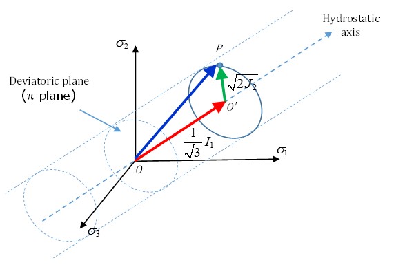
Рисунок 206: Напряженное состояние P

Масштаб O’P равен:

\[\sqrt{2J_{2}}=\sqrt{\frac{2}{3}} \sigma_{VM} \tag{156}\]

Здесь \(J_{2}\) — второй инвариант девиаторного напряжения \(\mathbf{s(s=\sigma-p)}\) с

\(J_{2}=\frac{1}{2}(S_{1}2+S_{2}2+S_{3}2)=\frac{1}{2}\Big{[}\big{(}\sigma_{1}-\sigma_{2}\big{)}^{2}+\big{(}\sigma_{2}-\sigma_{3}\big{)}^{2}+\big{(}\sigma_{3}-\sigma_{1}\big{)}^{2}\Big{]}\).

Чтобы определить точку P, необходимо вычислить угол в круговой плоскости. Этот угол называется углом Лоде \(\theta\): .. math:: cosbig{(}3thetabig{)}=frac{27}{2}frac{J_{3}}{sigma_{VM}^{3}}=frac{3sqrt{3}}{2}frac{J_{3}}{J_{2}^{3/2}} tag{157}

с \(0\leq\theta\leq\frac{\pi}{3}\) и \(J_{3}\) третий инвариант девиаторного напряжения, вычисляемый как:

\[J_{3}=S_{1}S_{2}S_{3} \tag{158}\]

В /FAIL/TAB1 нормализованный и безразмерный параметр угла Лоде \(\zeta\) с диапазоном \((-1\leq\zeta\leq 1)\) используется и определяется как:

\[\zeta=\cos\left(3\theta\right) \tag{159}\]

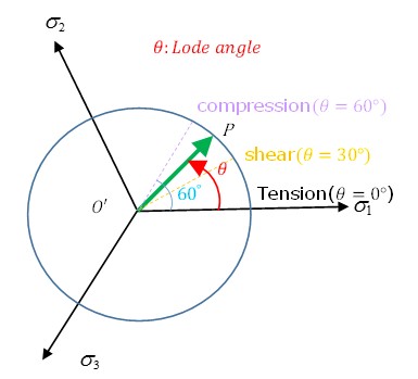
Рисунок 207: Напряженное состояние с различным углом нагрузки

Специальный символ для угла нагрузки \(\theta\) и параметра угла нагрузки \(\zeta\):

параметр угла нагрузки \(\zeta\)	угол жилы \(\theta\)	Страсс Стэйт
1	0	Одноосное растяжение+ гидростатическое давление (трехосное растяжение или осесимметричное растяжение )
0	30	Чистый сдвиг + гидростатическое давление (плоская деформация) n)
-1	60	Одноосное сжатие + гидростатическое давление (осесимметричное сжатие)

Поверхность деформации разрушения может быть создана на основе данных о трехосности напряжения и угле разрушения Лоде.

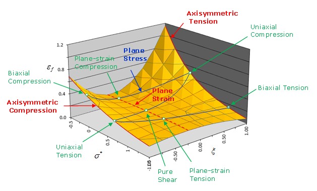
Рисунок 208: 3D-поверхность разрушения

Поверхность разрушения материала может быть создана с использованием следующих испытаний материалов. .. image:: vertopal_75794439f47d439ba01f734ac3f4dcc1/media/image8315.jpg

width

6.28387in

height

4.00868in

Рисунок 209: Состояние напряжения и угол нагрузки для различных испытаний

Пример /ТАБЛИЦА, размерность=3

Входные данные для пластической деформации разрушения в зависимости от трехосности, скорости деформации и угла нагрузки с использованием table_ID₁

/TABLE/1/4711
failure plastic-strain vs triaxiality and strain rate
#dimension
         3

#---1----|----2----|----3----|----4----|----5----|----6----|----7----|----8----|----9----|---10----|
# FCT_ID                      strain_rate           Lode_angle
    3000                            1E-4                   -1
    3001                             0.1                    0
    3002                             1.0                    1
. . . . . . . . .

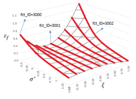
Рисунок 210: Поверхность разрушения, когда table_ID1 ссылается на * ``/TABLE`` *с размером=3

Масштабирование деформации разрушения

Разрушение материала на основе температуры и размера элемента можно рассмотреть в /FAIL/TAB1, включив функции, которые масштабируют деформацию разрушения в зависимости от размера элемента и/или температуры используя:

\[\varepsilon_{f}=Xscale1\cdot f(\sigma^{*},\xi,\xi)\cdot factor_{el}\cdot factor_{T} \tag{160}\]

Где

Xscale1 Общий коэффициент масштабирования

\(factor_{el}\) Коэффициент масштабирования на основе размера элемента

\(factor_{T}\) Коэффициент масштабирования на основе температуры

Зависимость длины элемента

В численном моделировании размер элемента будет влиять на разрушение материала. При использовании тех же параметров разрушения грубая сетка выйдет из строя раньше, чем мелкая. .. image:: vertopal_75794439f47d439ba01f734ac3f4dcc1/media/image87.jpg

width

3.50997in

height

2.44761in

Рисунок 211: Влияние размера сетки элемента на разрушение материала в численном моделировании

Чтобы учесть вариацию результатов в зависимости от размера сетки, можно определить масштабный коэффициент размера элемента для масштабирования деформации разрушения на основе размера элемента сетки. Масштабный коэффициент, определенный в уравнении 160, равен:

\[factor_{el}=Fscale_{el}\cdot\mathsf{f}_{el}\Big{(}\frac{Size_{el}}{EI_{-}ref} \Big{)} \tag{161}\]

Где,

\(F scale_{el}\) Масштабный коэффициент функции размера элемента \(\mathsf{f}_{el}\Big{(}\frac{Size_{el}}{EI_{-}ref}\Big{)}\) масштабный коэффициент деформации разрушения как функция нормализованного размера элемента (определяется через \(fct_ID_{el}\)), а EI_ref - это размер опорного элемента, используемый для нормализации размера элемента

Например, размер сетки 2 мм использовался в моделировании проверки материала. После первоначальной проверки та же симуляция перезапускается используя EI_ref = 2 с разными размерами элементов, чтобы определить правильный масштабный коэффициент для каждого размера элемента. Используя результаты второй проверки, функция масштабного коэффициента деформации разрушения строится как (рисунок 212):

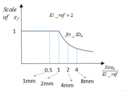
Рисунок 212: Пример функции масштабного коэффициента размера элемента fct_IDel in /FAIL/TAB1

Зависимость от температуры

Чтобы учесть, как температура влияет на разрушение материала, значения деформации разрушения, определенные в уравнении 160, можно масштабировать с помощью функции масштабного коэффициента температуры:

\[factor_{T}=Fscale_{T}\cdot\mathrm{f}_{T}(T_{start}) \tag{162}\]

Где,

\(F scale_{T}\) Коэффициент масштабирования температурной функции

\(\mathrm{f}_{T}(T_{start})\) Коэффициент масштабирования деформации разрушения как функция температуры, определяемая через \(fct_ID_{T}\)

Масштабирование деформации разрушения на основе температуры работает с любым материалом, у которого определен /HEAT/MAT или материалами, которые включают термопластичность, например, /MAT/LAW2 (PLAS_JOHNS).

В \(fct_ID_{T}\) температура определяется относительно плавления и начальной температуры.

\[T^{*}=\frac{T-T_{ini}}{T_{melt}-T_{ini}} \tag{163}\]

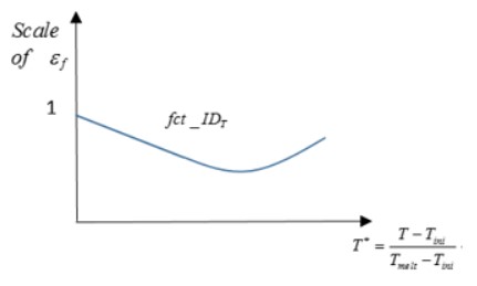
Рисунок 213: Влияние температуры на разрушение материала с fct_IDT в /FAIL/TAB1

Обработка разрушения элемента

В /FAIL/TAB1 используется модель накопленного повреждения. Повреждение может быть выведено для контурного построения с использованием параметров движка, /ANIM/SHELL/DAMA или /ANIM/BRICK/DAMA.

Накопленное повреждение рассчитывается путем предварительного расчета приращения повреждения: .. math:: Delta D=frac{Delta E_{p}}{varepsilon_{f}}cdot ncdot D_{p}(frac{1}{n})tag{164}

Где,

\(\Delta\varepsilon_{p}\) Изменение пластической деформации точки интегрирования

\(\varepsilon_{f}\) Пластическая деформация разрушения для текущего напряжения трехосность

\(D_{p}\) и n Параметры повреждения

Накопленное повреждение:

\[D=\frac{\sum_{\Delta D}}{D_{crit}}\tag{165}\]

Где, \(D_{crit}\) определено в /FAIL/TAB1 с рекомендуемым значением от 0 до 1. Элементы выходят из строя, когда \(D\geq 1\), что означает, \(\sum\Delta D\geq D_{crit}\). .. image:: vertopal_75794439f47d439ba01f734ac3f4dcc1/media/image9-0.jpg

width

5.97842in

height

4.05158in

Рисунок 214: Влияние \(D_{crit} на\) * /FALL/TAB1

Также интересно понять влияние параметра накопления повреждений в уравнении 164.

Когда *n*=1 повреждение линейно, в противном случае кривая повреждения нелинейна.

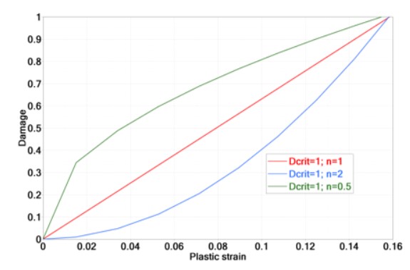
Рисунок 215: Влияние параметра повреждения *n

Нестабильность материала (диффузное сужение)

В испытании на растяжение материал достигает максимального инженерного напряжения, а затем напряжение уменьшается или иногда называется размягчается. Эта максимальная точка инженерного напряжения называется точкой сужения. После ссужения истинное напряжение фактически увеличивается из-за уменьшения площади поперечного сечения. Это называется диффузным сужением. В листовом металле может возникнуть утончение толщины или локальное сужение в диффузной области, если материал продолжает нагружаться в направлении растяжения. Диффузное сужение обычно появляется в диапазонах трехосности напряжений \(0<\sigma^{*}\leq\frac{2}{3}\) и локальное сужение в диапазоне \(\frac{1}{3}\leq\sigma^{*}\leq\frac{2}{3}\).

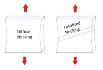
Рисунок 216: Эскиз диффузного шейкообразования и локализованного

В /FAIL/TAB1 можно учесть нестабильность материала (диффузное шейкообразование) с параметрами table_ID₂ или Inst_start и *Fad_exp

Материал начнет ослабевать из-за диффузного шейкообразования, когда будет достигнута деформация нестабильности. Приведенное напряжение в материале:

\[\sigma_{reduced}=\sigma\cdot\left(1-\left(\frac{D_{instability}-inst_start}{1- inst_start}\right)^{Fad_exp}\right)\tag{166}\]

Где,

\[D_{instability}=\sum\frac{\Delta\varepsilon_{p}}{\varepsilon_{f}}\tag{167}\]

с \(\varepsilon_{f}\) будучи диффузной деформацией шейки основанной на текущей напряженной триаксиальности.

Деформация, при которой начинается нестабильность, может быть либо введена с помощью кривой (синяя кривая на рисунке 217) с использованием table_ID₂, либо введена как ограниченная деформация с использованием опции Inst_start.

В одноосном испытании на растяжение \(\sigma^{*}=\frac{1}{3}\).

• Если нестабильность материала не включена, то повреждение рассчитывается с использованием красной кривой разрушения на рисунке 217

• Если нестабильность материала включена и смоделирована с использованием входной кривой (table_ID₂), то:

• Повреждение из-за диффузного образования шейки начинается, когда достигается пластическая деформация, определяемая синей кривой на рисунке 217.

• Повреждение из-за диффузного сужения линейно, если используется Fad_exp=1. Увеличение Fad_exp приводит к большему рассеиванию энергии во время повреждения. На рисунке 217 показано влияние Fad_exp от 1 до 10 на кривую напряжения-деформации. Рекомендуется использовать значение Fad_exp от 5 до 10.

• Как только деформация достигает красной кривой, элемент выходит из строя.

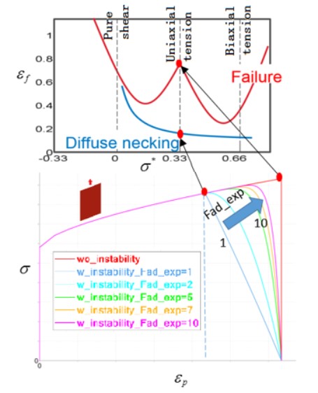
Рисунок 217: Влияние параметра Fad_exp и области нестабильности материала

• Если используется только Inst_start без ввода кривой в table_ID₂, то пластическая деформация диффузного сужения является постоянным значением, Inst_start, для всех напряжений трехосности.

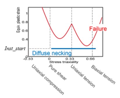
Рисунок 218: Константа Inst_start, описывающая диффузное шейкообразование

В настоящее время диффузное шейкообразование (нестабильность материала) в /FAIL/TAB1 может использоваться только с числами законов материалов > 28.

14. Вежбицкий, Томаш, “Дополнение к исследовательскому предложению по разрушению усовершенствованных высокопрочных сталей”, стр. 19, январь 2007 г.

15. Вежбицкий, Томаш. “Разрушение листов AHSS–Дополнение к исследовательскому предложению по разрушению усовершенствованных высокопрочных сталей”. Лаборатория ударопрочности и ударопрочности, Массачусетский технологический институт (2007 г.).

Композиты

Композитные материалы состоят из двух или более материалов, объединенных друг с другом. Большинство композитов состоят из двух материалов: связующего (матрицы) и армирования. Армирование бывает трех видов: частичные, прерывистые волокна и непрерывные волокна.

Композитный материал

В PRADIOS для описания композитного материала используются следующие законы материалов:

• LAW12 и LAW14

• LAW15 (рекомендуется использовать LAW25+/FAIL/CHANG)

• LAW25

• LAW19 (Для ткани и только с /PROP/TYPE9)

• LAW58 (Только для ткани с``/PROP/TYPE16``)

Таблица 19: Композитный материал, свойство, модель отказа и совместимость типов элементов

	Элемент оболочки	Элемент кирпича	Модель отказа
LAW12		/PROP/TYPE6 (SOL_ORTH) /PROP/TYPE21 (TSH_ORTH) /PROP/TYPE22 (TSH_COMP)	/FAIL/HASHIN /FAIL/PUCK /FAIL/LAD_DAMA
LAW14		/PROP/TYPE6 (SOL_ORTH) /PROP/TYPE21 (TSH_ORTH) /PROP/TYPE22 (TSH_COMP)	/FAIL/HASHIN /FAIL/PUCK /FAIL/LAD_DAMA
LAW15	/PROP/TYPE9 (SH_ORTH) /PROP/TYPE10 (SH_ORTH) /PROP/TYPE11 (SH_SANDW) /PROP/TYPE17 (STACK) /PROP/TYPE19 (PLY)		/FAIL/CHANG
LAW25	/PROP/TYPE10 (SH_ORTH) /PROP/TYPE11 (SH_SANDW) /PROP/TYPE17 (STACK) /PROP/TYPE19 (PLY) /PROP/TYPE51 /PROP/PCOMPP	/PROP/TYPE6 (SOL_ORTH) /PROP/TYPE14 (SOLID) /PROP/TYPE20 (TSHELL) /PROP/TYPE21 (TSH_ORTH) /PROP/TYPE22 (TSH_COMP)	/FAIL/CHANG /FAIL/HASHIN /FAIL/PUCK /FAIL/LAD_DAMA (for solid only)
LAW19	/PROP/TYPE9 (SH_ORTH)
LAW58	/PROP/TYPE16 (SH_FABR)

LAW12 и LAW14

Описывает ортотропный твердый материал, который использует формулировку Цая-У. Материалы являются 3D ортотропно-упругими, до достижения критерия Цая-У. LAW12 является обобщением и улучшением LAW14.

Упругая фаза

Оба закона материала требуют модуль Юнга, модуль сдвига и коэффициент Пуассона (9 параметров) для описания ортотропного материала в упругой фазе. .. image:: vertopal_75794439f47d439ba01f734ac3f4dcc1/media/image9-5.jpg

width

3.50864in

height

1.1251in

Рисунок 219:

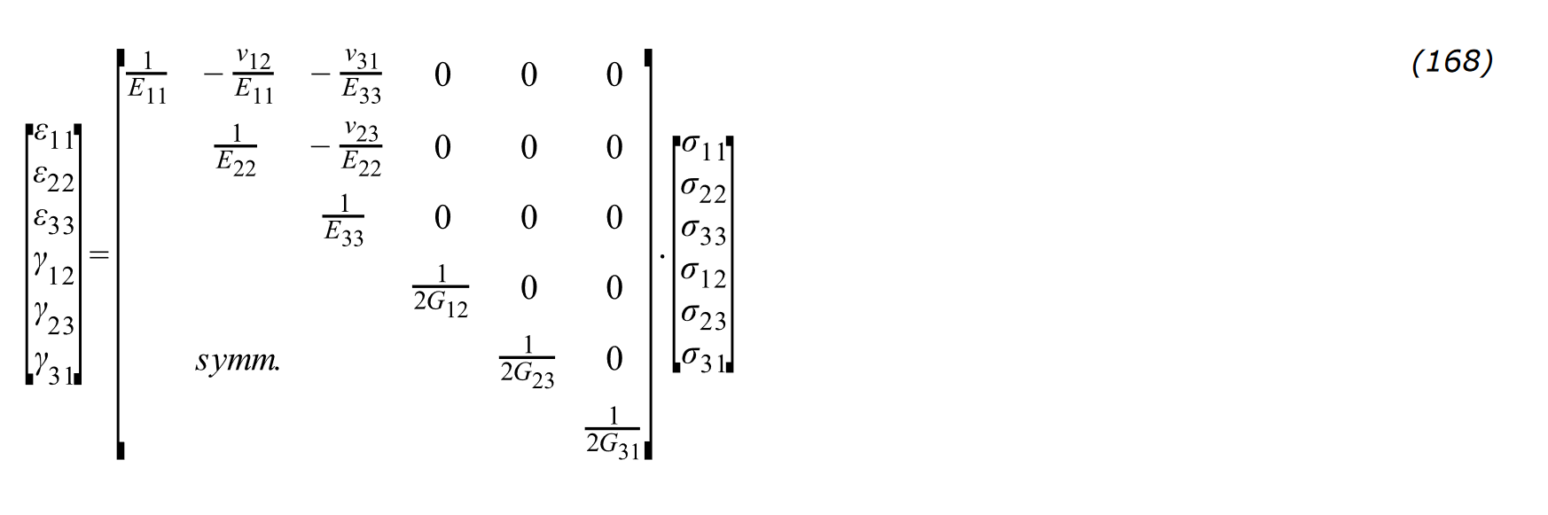
Стрессовое повреждение

Рисунок 220:

Пределы напряжения \(\sigma_{t1}\) и \(\sigma_{t2}\) и \(\sigma_{t3}\) (при растяжении/сжатии) запрашиваются для повреждения. Эти пределы напряжения можно было бы наблюдать из испытания на растяжение в 3 связанных направлениях.

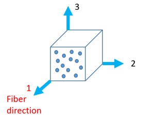
Рисунок 221:

После достижения предела напряжения начинается повреждение материала (напряжение уменьшается параметром повреждения \(\sigma\)). Если Ущерб (\(D_{i}=D_{i}+\sigma)\) достигает D=1, то напряжение уменьшается до 0.

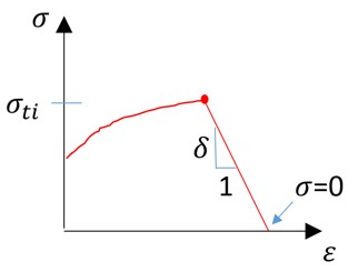
Рисунок 222:

Критерии доходности Цай-У

В LAW12 (3D_COMP) критерий доходности Цай-У:

\[F(\sigma)=F_{1}\sigma_{1}+F_{2}\sigma_{2}+F_{3}\sigma_{3}+F_{1}\sigma_{1}^{2}+F_{2}\sigma_{2}^{2}+F_{3}\sigma_{3}^{2}+F_{4}\sigma_{12}^{2}+F_{5}\sigma_{23}^{2}+F_{6}\sigma_{3}^{2}+2F_{1}\sigma_{1}\sigma_{2}+2F_{2}\sigma_{2}\sigma_{3}+2F_{1}\sigma_{1}\sigma_{3} \tag{169}\]

12 коэффициентов критерия Цая-У можно определить, используя предел текучести из следующих испытаний:

Испытания на растяжение/сжатие

• Продольное растяжение/сжатие (в направлении 1):

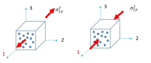
Рисунок 223: .. math:: F_{1}=-frac{1}{sigma_{rm ly}^{c}}+frac{1}{sigma_{rm ly}^{t}} tag{170}

\[F_{1}=\frac{1}{\sigma_{\rm ly}^{c}\sigma_{\rm ly}^{t}}\tag{171}\]

• Поперечное растяжение/сжатие (в направлении 2):

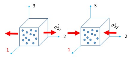
Рисунок 224:

\[F_{2}=-,\frac{1}{\sigma_{2y}^{c}}+\frac{1}{\sigma_{2y}^{t}}\tag{172}\]

\[F_{22}=\frac{1}{\sigma_{2y}^{c}\sigma_{2y}^{t}}\tag{173}\]

• Поперечное растяжение/сжатие (в направлении 3):

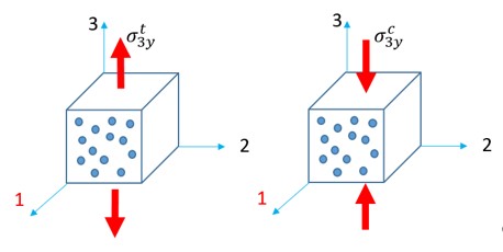
Рисунок 225:

\[F_{3}=-,\frac{1}{\sigma_{3y}^{c}}+\frac{1}{\sigma_{3y}^{t}}\tag{174}\]

\[F_{33}=\frac{1}{\sigma_{3y}^{c}\sigma_{3y}^{t}}\tag{175}\]

Тогда коэффициенты взаимодействия можно рассчитать как: .. math:: F_{12}=-,frac{1}{2}sqrt{left(F_{11}F_{22}right)}tag{176}

\[F_{23}=-,\frac{1}{2}\sqrt{\left(F_{22}F_{33}\right)}\tag{177}\]

\[F_{13}=-,\frac{1}{2}\sqrt{\left(F_{11}F_{33}\right)}\tag{178}\]

Испытания на сдвиг

• Испытание на сдвиг в плоскости 1-2:

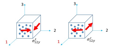
Рисунок 226:

\(\sigma^{t}_{12y}\), и \(\sigma^{c}_{12y}\) могут быть получены из приведенных ниже примеров тестов:

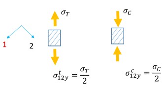
Рисунок 227:*

\[F_{44}=\frac{1}{\sigma^{c}_{12y}\sigma^{t}_{12y}}\tag{179}\]

• Сдвиг в плоскости 1-3

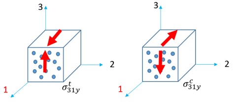
Рисунок 228:

\(\sigma^{t}_{3,1y}\) и \(\sigma^{c}_{3,1y}\), могут быть получены из приведенных ниже примеров тестов: .. image:: vertopal_75794439f47d439ba01f734ac3f4dcc1/media/image10-5.jpg

width

3.04193in

height

1.63347in

Рисунок 229:

\[F_{66}=\frac{1}{\sigma_{31y}^{c}\sigma_{31y}^{t}}\tag{180}\]

• Сдвиг в плоскости 2-3:

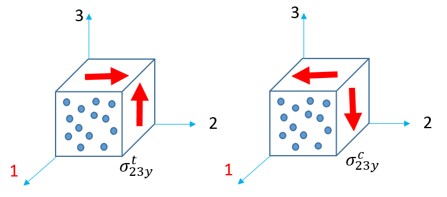
Рисунок 230:

\[F_{55}=\frac{1}{\sigma_{23y}^{c}\sigma_{23y}^{t}}\tag{181}\]

Параметры, показанные ниже в LAM12 и LAM14, требуются для расчета критериев Цая-У:

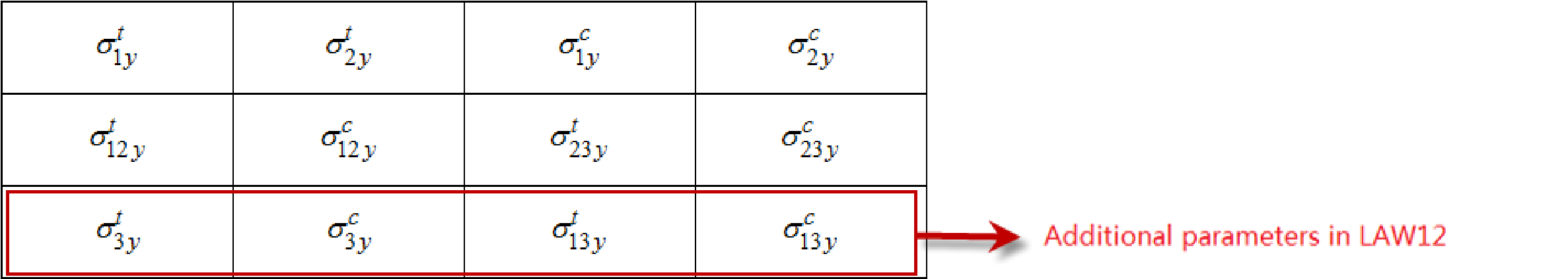
Рисунок 231:

Поверхность текучести для Цая-У равна \(F(\sigma)=1\). Пока \(\left(F(\sigma)\leq 1\right)\), материал находится в упругой фазе. Как только \(\left(F(\sigma)>1\right)\), поверхность текучести превышена, и материал находится в нелинейной фазе.

В этих двух материальных законах следующие факторы также могут быть рассмотрены для поверхности текучести.

• Пластическая работа \(W_{p}\) с параметрами B и n

• Скорость деформации \(\dot{\varepsilon}\) с параметром \(\dot{\varepsilon}_{0}\) и c.

\[F\big{(}W_{p},\dot{\varepsilon}\big{)}=\big{(}1+BW_{p}^{n}\big{)}\Big{(}1+c\mathrm{ln}\frac{\dot{\varepsilon}}{\dot{\varepsilon}_{0}}\Big{)}\tag{182}\]

Тогда поверхность текучести будет \(F(\sigma)=F\big{(}W_{p},\dot{\varepsilon}\big{)}\).

• Материал будет в упругой фазе, если \(F(\sigma)\leq F\big{(}W_{p},\dot{\varepsilon}\big{)}\)

• Материал будет в нелинейной фазе, если \(F(\sigma)>F\big{(}W_{p},\dot{\varepsilon}\big{)}\)

Эта поверхность текучести \(F\big{(}W_{p},\dot{\varepsilon}\big{)}\) будет ограничена \(f_{\mathrm{max}}(F\big{(}W_{p},\dot{\varepsilon}\big{)}\leq f_{\mathrm{max}})\), где \(f_{\mathrm{max}}\) - максимальное значение Tsai-Wu предел критерия.

\(f_{\mathrm{max}}=\Big{(}\frac{\sigma_{\mathrm{max}}}{\sigma_{y}}\Big{)}^{2}\)

В зависимости от параметров B, n, c и \(\dot{\varepsilon}_{0},\) поверхность текучести находится между 1 и \(f_{\mathrm{max}}\).

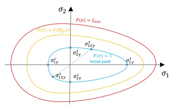
Рисунок 232: Критерии текучести Цая-Ву в плоскости 1-2

LAW25 (Tsai-WU и CRASURV)

LAW25 — наиболее часто используемый композитный материал в PRADIOS. Его можно использовать с оболочечными и твердыми элементами. Две формулы, доступные в LAW25, — это формулы Цая-Ву и CRASURV.

Упругая фаза

В упругой фазе для описания ортотропного материала требуются модуль Юнга (3 параметра), модуль сдвига (3 параметра) и один параметр для коэффициента Пуассона.

Критерии текучести Цая-У для \(\mathbf{I_{form}}\) =0 и =1

Поверхность текучести Цая-У в LAW25 определяется с 6 коэффициентами:

\(\mathbf{I_{form}}\) : Цай-У \(\mathbf{I_{form}}\) : CRASURV \(\left(F(W^{*}_{\mathbf{p}},\varepsilon,\sigma)\leq 1\right)\)

\(\left(F(\sigma)\leq F(W^{*}_{\mathbf{p}},\varepsilon)\right)\)

Чтобы проверить, находится ли материал в текучести, в Цай-У (\(I_{form}\) будет сравниваться с \(F(W^{*}_{\mathbf{p}},\varepsilon)\) в каждом напряженном состоянии и в CRASURV (\(I_{form}=1)\) \(F(W^{*}_{\mathbf{p}},\varepsilon)\) будет просто сравниваться с 1 в каждом напряженном состоянии. Эти 6 коэффициентов можно определить с пределом текучести из этих испытаний:

• Испытания на растяжение/сжатие

Испытания на продольное растяжение/сжатие (в направлении 1, которое является направлением волокон):

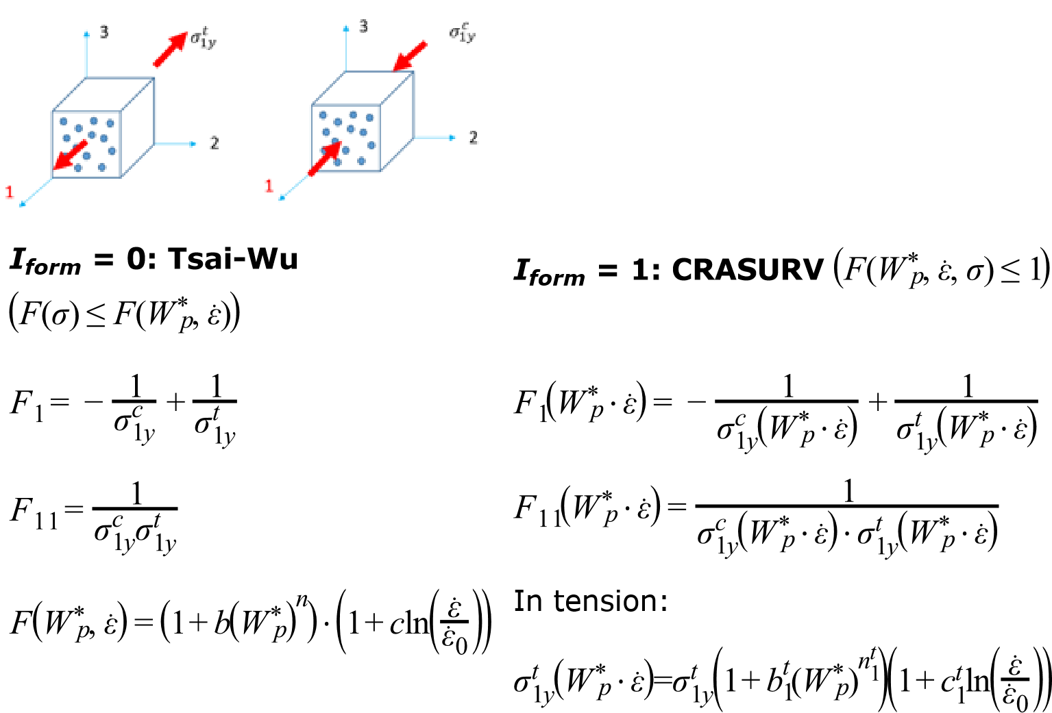
Здесь \((W^{*}_{p}=\frac{W_{p}}{W^{ref}_{p}})\) в сжатии:

\(\sigma^{c}_{1y}\big{(}W^{*}_{p}\cdot\varepsilon\big{)}=\sigma^{c}_{1y}\big{(}1+b^{c}_{1}\big{(}W^{*}_{p}\big{)}^{n^{c}_{1}}\big{(}1+c^{c}_{1}\ln\Big{(}\frac{\varepsilon}{\varepsilon_{0}}\Big{)}\big{)})\)

Здесь \((W^{*}_{p}=\frac{W_{p}}{W^{ref}_{p}})\)

Испытания на поперечное растяжение/сжатие (в направлении 2) .. image:: vertopal_75794439f47d439ba01f734ac3f4dcc1/media/image11-1.png

width

6.11667in

height

4.47in

• Испытания на сдвиг

Сдвиг в плоскости 1-2 .. image:: vertopal_75794439f47d439ba01f734ac3f4dcc1/media/image1-1-2.jpg

width

6.11667in

height

6.47in

\(I_{form}\) = 0: Tsai-WU \(\left(F(\sigma)\leq F(W^{*}_{\mathbf{p}},\varepsilon)\right)\)

\(I_{form}\) = 1: CRASURV \(\left(F(W^{*}_{\mathbf{p}},\varepsilon,\sigma)\leq 1\right)\)

\(F_{12}=-\frac{a}{2}\sqrt{F_{11}F_{22}}\)

Обычно используется коэффициент уменьшения по умолчанию, a-1.

\(F\big{(}W_{p}^{*},\dot{\varepsilon}\big{)}=\big{(}1+b \big{(}W_{p}^{*}\big{)}^{n}\big{)}\cdot\Big{(}1+\mathrm{cln}\big{(}\frac{\dot{\varepsilon}}{\dot{\varepsilon}_{0}}\big{)}\Big{)}\)

Здесь, \((W^{*}_{p}=\frac{W_{p}}{W^{ref}_{p}})\)

\(F_{12}\big{(}W_{p}^{*},\dot{\varepsilon}\big{)}=-\frac{a}{2}\sqrt{F_{11}\big{(}W_{p}^{*},\dot{\varepsilon}\big{)}F_{22}\big{(}W_{p}^{*},\dot{\varepsilon}\big{)}}\)

Обычно используется коэффициент уменьшения по умолчанию, a-1.

Обратите внимание, что относительная пластическая работа \(W_{p}^{*}\) используется в Tsai-WU для расчета поверхности текучести; тогда как в CRASURV для расчета предела текучести используется относительная пластическая работа. .. image:: vertopal_75794439f47d439ba01f734ac3f4dcc1/media/Untitl3422ed.png

width

6.71667in

height

5.47in

Предел текучести \(F(W^{*}_{\mathbf{p}},\varepsilon)\) находится в диапазоне от 1 до \(f_{max}\)

В LAW25 (Tsai-Wu и CRASURV) повреждение является функцией общей деформации и максимального фактора повреждения.

Если общая деформация \(\varepsilon>\varepsilon_{t}\) или внеплоскостная деформация \(\gamma_{ini}<\gamma<\gamma_{\max}\), то материал смягчается с использованием следующего метода:

\[\sigma^{reduce}=\sigma\cdot(1-d_{i})\tag{184}\]

при i =1,2,3

Где, \(d_{i}\) — фактор повреждения, который определяется как:

\[d_{i}=\min\left(\frac{\varepsilon_{i}-\varepsilon_{ti}}{\varepsilon_{i}}\cdot\frac{\varepsilon_{ini}}{\varepsilon_{ini}}, d_{\max}\right)\tag{185}\]

при i =1,2

\[d_{3}=\min\left(\frac{\gamma-\gamma_{ini}}{\gamma_{\max}-\gamma_{ini}}\cdot\frac{\gamma_{\max}}{\gamma},d_{\max}\right)\tag{186}\]

в направление 3 (расслоение)

• Если общая деформация находится в пределах \(\varepsilon_{t}<\varepsilon_{t}<\varepsilon_{f}\), материал начинает размягчаться, но это повреждение обратимо. Как только \(\varepsilon>\varepsilon_{f}\), повреждение становится необратимым, а если \(\varepsilon\geq\varepsilon_{m})\), напряжение в материале снижается до 0.

• Повреждение может быть в упругой фазе или в пластической фазе. Это зависит от того, в какой фазе определены \(\varepsilon_{t}\) и \(\varepsilon_{f}\).

• Удаление элемента контролируется \(I_{\mathit{off}}\). Выберите другой параметр \(I_{\mathit{off}}\) для управления критериями удаления элемента. Для получения дополнительной информации см. \(I_{\mathit{off}}\) в LAW25 в Справочном руководстве.

LAW19 и LAW58 для ткани

PRADIOS имеет два закона материалов для моделирования тканей LAW19 и LAW58. LAW19 — это эластичный ортотропный материал, который необходимо использовать с /PROP/TYPE9. LAW58 — это гиперэластичный анизотропный материал ткани, который необходимо использовать с /PROP/TYPE16.

В этом законе материалов можно определить связь между направлениями основы и утка для воспроизведения физического взаимодействия между волокнами. Оба закона материалов часто используются для моделирования подушек безопасности.

В LAW58 предусмотрено два метода для определения поведения напряжения-деформации.

• Нелинейная функция (\(fct\_ID_{i}\)) кривая для определения поведения основы, утка и сдвига

• Модуль Юнга, коэффициент размягчения (B), деформация выпрямления \(S_{i}\) и коэффициент уменьшения модуля изгиба волокна \(\mathit{Flex}_{i}\)

  В направлении основы и утка: \(\sigma_{ii}=E_{i}\varepsilon_{ii}-\frac{(B_{i}\varepsilon_{ii})}{2}\quad(i=1,2)\text{когда}\frac{d\sigma}{d\varepsilon}>0\)

  \(\sigma_{ii}=\max_{\varepsilon_{ii}}\left(E_{i}\varepsilon_{ii}-\frac{(B_{i}\varepsilon_{ii})}{2}\right)\quad(i=1,2)\text{когда}\frac{d\sigma}{d\varepsilon}\leq 0\)

  Для сдвига в плоскости в исходном состоянии используйте \(G_{0}\). Как только \(\alpha\) (угол между обмоткой и утком)

достигнет \(\alpha_{T}\) (угол фиксации сдвига), используйте \(G_{T}\) для описания усиления.

\(\tau=G_{0}\text{tan}(\alpha)-\tau_{0}\text{if}\alpha\leq\alpha_{T}\)

\(\tau =\frac{G_{T}}{1+\tan^{2}(\alpha_{T})}\text{tan}(\alpha)+\left(G_{0}-\frac{G_{T}}{1+\tan^{2}(\alpha_{T})}\right)\text{tan}(\alpha_{T})-\tau_{0}\text{if}\alpha>\alpha_{T}\)

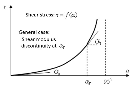
Рисунок 233:*

Для напряжения сдвига вне плоскости описывается с помощью \(G_{sh.}\)

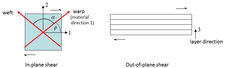
Рисунок 234:

Для ткани в начале натяжения наблюдается прямой процесс. На этой фазе волокно выглядит очень мягким, так как еще не натянуто. .. image:: vertopal_75794439f47d439ba01f734ac3f4dcc1/media/image1-18.jpg

width

3.917in

height

1.39179in

Рисунок 235:

В LAN58 используйте \(Flex_{i}\) для описания этого поведения:

\[E_{fi}=Flex_{i}*E_{i} \tag{187}\]

После того, как ткань станет плотной (упрочняющая деформация \(S_{i}\) будет достигнута), тогда может быть достигнута нормальная эластичность волокна \(E_{i}\).

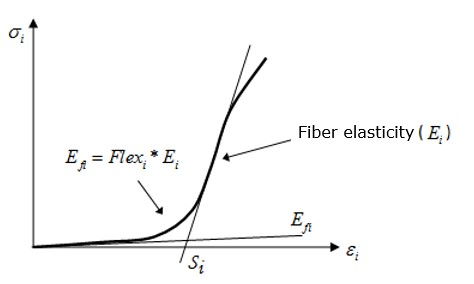
Рисунок 236:

Композитное моделирование

Технологии композитного моделирования, используемые в PRADIOS.

Каждый слой с по крайней мере одним твердым телом

Модель большая, что приводит к результатам высокой точности, но требует больше вычислительных ресурсов.

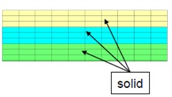
Рисунок 237:

Смешанный подход (средний слой толстый)

Определяет оболочки для верхнего и нижнего слоя и твердое тело для среднего слоя.

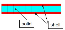
Рисунок 238:

Подход сэндвич-оболочкой

Используйте только один элемент оболочки по всей толщине. Используйте разные материалы для определения нескольких слоев. .. image:: vertopal_75794439f47d439ba01f734ac3f4dcc1/media/image12-2.jpg

width

1.95017in

height

0.7834in

Рисунок 239:

В моделировании композитных оболочек есть два типа проблем.

• Первый тип - композитная оболочка с изотропными слоями (ортотропными в направлении z). Например, моделированием ветрового стекла. Где можно использовать материал LAW27(PLAS_BRIT) или LAW36 (PLAS_TAB).

• Второй тип - композитная оболочка с ортотропными слоями (ортотропными в x, y и z). Например, сэндвич-оболочка с внешними слоями стекловолокна и внутренним слоем пены. Где можно использовать материал LAW25 (COMPSH) и все формулы оболочек, за исключением QEPH.

Свойства композита

Композит может быть смоделирован с помощью твердого или оболочечного элемента. В зависимости от типа элемента в PRADIOS можно использовать следующие свойства для моделирования композита.

Элементы оболочки

Моделирование композита в PRADIOS может быть определено на основе слоев или на основе слоев с различными свойствами. - Моделирование на основе слоев с помощью /PROP/TYPE10 (SH_COMP), /PROP/TYPE11 (SH_SANDW)

• Моделирование на основе слоев с /PROP/TYPE17 (STACK), /PROP/TYPE51, /PROP/PCOMPP+/STACK, /PROP/ TYPE19 (PLY) and /PLY

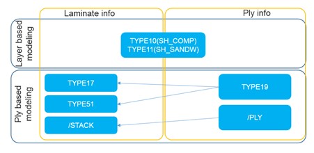
Рисунок 240:

Для моделирования на основе слоев информация (например, материал, толщина, анизотропный угол, анизотропный угол оси и количество точек интегрирования) для каждого слоя, определенного в /PROP/TYPE19 (или /PLY) и собранного в /PROP/ TYPE17 или /PROP/TYPE51 (или /STACK) с опцией Pply_\(D_{i}\). .. image:: vertopal_75794439f47d439ba01f734ac3f4dcc1/media/image124.jpg

width

6.84226in

height

2.18353in

Рисунок 241:

Для моделирования на основе слоев способ сборки слоев может быть «по слою» или «по подстеку». «По слою» — это просто наложение слоев один за другим снизу вверх. Для способа «по подстеку» необходимо сначала накладывать слои один за другим, чтобы создать каждый подстек, а затем каждый подстек может быть либо объединен, либо также может быть сложен с помощью соединения подстека «INT». .. image:: vertopal_75794439f47d439ba01f734ac3f4dcc1/media/image125.jpg

width

6.7804in

height

2.6455in

Рисунок 242: .. image:: vertopal_75794439f47d439ba01f734ac3f4dcc1/media/image12-6.jpg

width

6.84289in

height

2.15599in

Рисунок 243: Стек в /PROP/TYPE51

Для составного свойства следующие темы:

• Количество слоев (прокладок) и точек интеграции каждого слоя (прокладки)

• Анизотропия в слое (ply)

• Толщина и положение слоя (прослойки)

• Композитный материал, используемый для слоя (ply)

Номер слоя (Ply) N (\(Nply\_ID_{i}\)) и точки интеграции каждого слоя (Ply)

Для моделирования на основе слоев, которое использует /PROP/TYPE10, /TYPE11. N — это количество слоев по толщине оболочки. Для этих свойств есть одна точка интеграции (IP) для каждого слоя.

Для моделирования на основе слоев, которое использует /PROP/TYPE17, /TYPE51 и /PCOMPP. Pply_ID — это количество слоев по толщине оболочки. Слои можно объединять до n слоев для этих свойств.

Для TYPE17 допускается только одна точка интеграции, а для TYPE51 и /STACKF допускается до 9 точек интеграции. Количество точек интеграции, определенных с помощью параметра «Npt_ply» в свойстве TYPE19 или /PLY.

Пример (Ply) (/PROP/TYPE51)

В этом примере Npi_ply=3, определенное в /PROP/TYPE19, означает 3 точки интегрирования, определенные для каждого слоя, и с опцией \(I_{int}\) =1, определенной в /PROP/TYPE51, эти 3 точки интегрирования равномерно распределены по толщине каждого слоя. каждой толщине слоя.

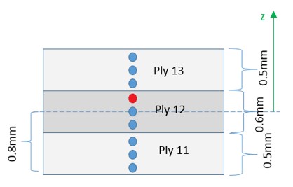
Рисунок 244:

Если \(I_{int}\) =1 в /PROP/TYPE51, то точки интегрирования распределяются в соответствии с расчетом сил и моментов Схемой интегрирования Гаусса по толщине каждого слоя.

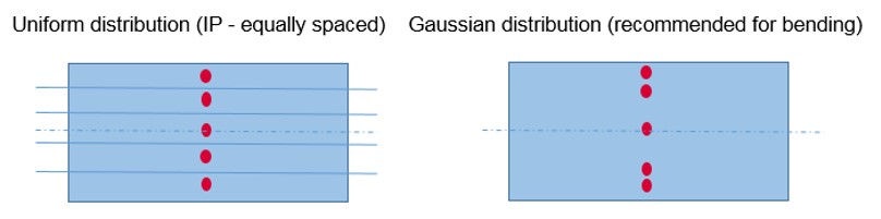
Рисунок 245:

Можно распечатать результаты анимации (пластическая деформация, повреждение, напряжение и тензор деформации) в каждой конкретной точке интеграции с /ANIM/SHELL/IDPLY/Keyword4/I/J (или /ANIM/SHELL/Keyword3/N/NIP).

Например, используйте /ANIM/SHELL/IDPLY/EPSP/2/3 (или /ANIM/SHELL/EPSP/2/3) для печати пластической деформации в третьей точке интеграции (красная выделенная точка интеграции на рисунке 245) второго слоя (имя слоя Ply12). Для получения дополнительной информации о печати точек интеграции через толщину оболочки для свойств композита см. Вывод тензора напряжения оболочки в анимации. в разделе часто задаваемых вопросов.

Анизотропия в слое (Ply)

• Первое анизотропное направление материала можно определить с помощью угла \(\phi\) и глобального вектора \(\mathbf{V}(V_{x}),(V_{Y}),(V_{Z})\). Также можно использовать угол \(\phi\) и перекос. В этом случае ось x перекоса заменила глобальный вектор \(\mathbf{V}\).

  Проецируем глобальный вектор \(\mathbf{V}\) на элемент оболочки и затем вращаем \(\phi\) степень — это первое анизотропное направление (также называемое направлением материала 1). Положительное направление \(\phi\) — это кодирование к нормали оболочки \(\mathbf{n}\). Например, на рисунке 246 вращаем против часовой стрелки \(\phi\) степень — это направление материала 1.

  Направление материала 1 локальной ссылки на элемент обычно является направлением волокна. Тогда материальный характер (модуль упругости, предел текучести и т. д.) направления 1, который определен в материальном праве, может быть затем применен в правильном направлении локальной ссылки на элемент.

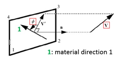
Рисунок 246:

• Композитный материал может быть ортотропным или анизотропным. В Radios можно описать этот характер с анизотропным углом оси \(\alpha_{i}\) в свойствах на основе слоев. В случае \(\alpha_{i}=90^{\circ}\), то он описывает ортотропный материал. Для свойств на основе слоев (TYPE10 и TYPE11), которые без этой опции \(\alpha_{i}\), так что можно определить только ортотропный материал.

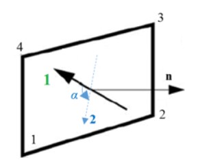
Рисунок 247:

На рисунке 248 показан пример в /PROP/TYPE11, который использует перекос для определения глобального вектора V.

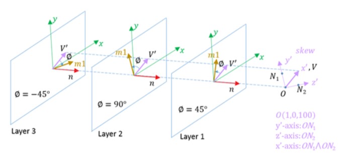
Рисунок 248:

Для свойств TYPE11 и TYPE51 анизотропное направление для некоторой оболочки также может быть инициализировано с помощью \(\phi\) в ключевом слове /INISHE/ORTH_LOC или /INISH3/ORTH_LOC. Для свойства TYPE51 анизотропный угол оси также может быть инициализирован с помощью этих ключевых слов.

• Ориентация анизотропии для определенных элементов оболочки или групп элементов оболочки может быть снова изменена с помощью параметра drape_ID и def_orth в

/PROP/TYPE19 и /PLY. drape_ID определен в /DRAPE. С помощью этой функции угол анизотропного направления может быть изменен с помощью \(\theta_{drape}\).

• Если использовать def_orth=1: Angle:

\(\phi_{r}\) косой или глобальный вектор \(\mathbf{V}\) будет проигнорировано. Возьмем локальную ось x оболочки как vector \(\mathbf{V}_{*}\) а затем повернуть \(\phi\) степень - это первое анизотропное направление. \(\phi_{s}\) (определено в /SHELL или /SH3N) учитывается при вычислении угла \(\phi\)..

\[\phi=\phi_{s}+\Delta\phi+\theta_{drape}\tag{188}\]

• Если использовать def_orth=2 (по умолчанию)

Спроецируйте глобальный вектор \(\mathbf{V}\) в элементе оболочки на вектор \(\mathbf{V}^{*}\) и затем поверните \(\phi\) степень — это первое анизотропное направление. Угол \(\phi\) вычисляется как:

\[\phi=\phi_{i}+\Delta\phi+\theta_{drape} \tag{189}\]

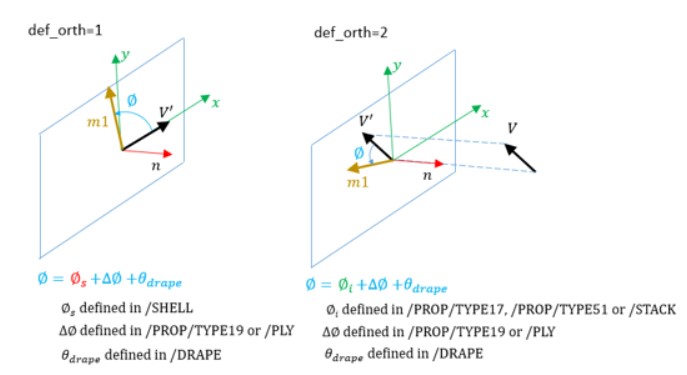
Рисунок 249:

Толщина и положение слоя (прослойки)

• Для /PROP/TYPE10 толщина слоя просто усредняется по номеру слоя

\[t_{i}=Thick/N \tag{190}\]

и слои автоматически накладываются друг на друга снизу вверх.

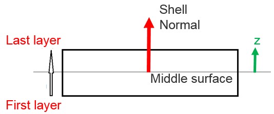
Рисунок 250:

• Для свойств TYPE11, TYPE17, TYPE51 и /STACK положение и толщина слоя (ply) зависят от параметра \(I_{pos}\)

◦ Если \(I_{pos}\) =0

Будет принят ввод толщины слоя (ply) пользователем, и положение слоя (ply) будет автоматически накладываться друг на друга снизу вверх; но если,

\[\sum_{i}t_{i}\neq Thick \tag{191}\]

Тогда толщина слоя (ply) будет скорректирована до \(t_{i}^{new}\), так что

\[\sum_{i}t_{i}^{new}= Thick \tag{192}\]

Положение слоя (ply) также будет скорректировано.

◦ если :math:`I_{pos}`=1

Пользовательский слой(ply) вводит толщину \(t_{i}\) и положение \(Z_{i}\). Сумма толщины слоя не будет проверяться с помощью (Thick).

Для получения дополнительной информации см. раздел Толщина слоя и расчет положения. в разделе часто задаваемых вопросов.

• Для свойств TYPE17, TYPE51 и /STACK также возможно смещение слоев с помощью :math:`I_{pos}`=2, 3, 4

• \(I_{pos}\) =2: срединная поверхность элемента оболочки находится на \(Z_{0}\) от нижней части макета слоя

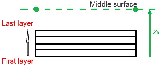
Рисунок 251:

• \(I_{pos}\) =3: верх слоя совпадает с поверхностью середины элемента

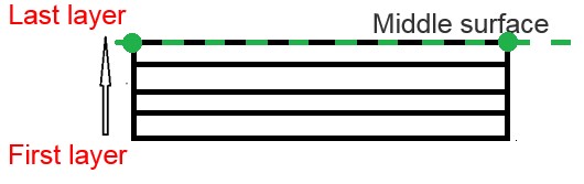
Рисунок 252:

• \(I_{pos}\) =4: нижняя часть слоя совпадает с поверхностью середины элемента

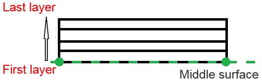
Рисунок 253:

• Для /PROP/TYPE17, /PROP/TYPE51 и /STACK толщина слоя может быть изменена с помощью параметра /DRAPE (который используется в /PROP/TYPE19 или /PLY). Тогда обновленная толщина слоя будет:

\[t_{i}^{new}=t_{i}\cdot Утончение \tag{193}\]

Композитный материал, используемый для слоя (Ply)

Композитный материал LAW15 и LAW25 можно использовать для элемента оболочки. Модель отказа /FAIL/HASHIN, /FAIL/PUCK и /FAIL/LAD_DAMA с LAW25 и /FAIL/CHANG с LAW15 можно использовать для описания композитного поведения элемента оболочки. Для получения дополнительной информации см. Композитный материал.

• Материал для слоя (ply)

  ◦ Для свойства TYPE10 композитный используемый материал определен в /PART

  ◦ Для свойств TYPE11 и TYPE17 композитный материал, определенный в опции mat_ \(ID_{i}\). Для каждого слоя (ply) можно задать разные идентификаторы материалов. Но они должны использовать один и тот же тип материала. Если используется LAW25, то для разных слоев (ply) можно использовать несколько разных карт LAW25.

  ◦ Для свойств TYPE51 и /STACK композит также использует материал, определенный в параметре mat_ \(ID_{i}\), и для каждого слоя можно использовать другой тип материала или идентификатор.

• Материал между слоями

  Для свойства TYPE17 можно определить расслоение между слоями или стопками (с Plyxfem=2). Это очень полезно, поскольку расслоение является основной причиной разрушения композита. Материал между слоями определяется с помощью Minterply. На данный момент LAW1+ /FAIL/LAD_DAM можно использовать для описания трех различных типов расслоения слоев.

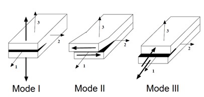
Рисунок 254:

И затем в этом случае дополнительная переменная :math:`_{1},_{2},_{3} добавляется к каждому узлу слоя по расчету для слоя по расчету для моделирования отказа от расслоения между слоями. .. image:: vertopal_75794439f47d439ba01f734ac3f4dcc1/media/im-age138.jpg

width

4.22864in

height

2.02058in

Рисунок 255:

Твердый элемент

Новая композитная технология позволяет вам производить детали больше и толще, так как моделирование этих деталей с помощью элементов оболочки недостаточно. Толстая оболочка может решить эту проблему. По сравнению с элементом оболочки, толстая оболочка может напрямую соединяться с другой твердотельной частью.

Для твердотельного элемента на данный момент доступно только послойное моделирование со свойством /PROP/TYPE22 (TSH_COMP). Это твердотельное свойство аналогично свойству оболочки /PROP/TYPE11 по определению композита.

	На основе слоев Характеристики
	/PROP/TYPE22 (TSH_COMP)
Номера слоев	\(I_{solid}\) =14: \(I_{int}\) =9~200	\(I_{solid}\) =15:
IP каждый слой/ прослойка	\(I_{npts}\) =ijk=2~9	\(I_{npts}\) =j=1~200
Интеграция формулировка
\(\phi_{i}\) + V, Анизотропное направление	√
\(\phi_{i}\) + перекос, Анизотропный направление	√
\(\theta_ {draper}\) , Ориентация слоя изменить
\(a_{i}\) , Угол между анизотропной осью
\(t_{i}\) , Слой/Прослойка толщина	√ определяется с фактором \(t_{i}/t\)
\(I_{pos}\) + \(Z_{i}\) Слой/Прослойка	√
\(I_{pos}\) =2,3,4, Слой/Прослойка компенсировать
\(mat\_ID_{i}\) , Материал для каждого Слой/Прослойка	√ Различные типы материалов позволяют каждый слой.
Обычно используется Композитный материал LAW	LAW12, LAW14, LAW25 и пользовательский материал
Plyxfem, Расслоение между слоем/слоем
Minterply, Material between Слой/Прослойка

• Номер слоя и точки интеграции каждого слоя

  Номер слоя, определенный с помощью параметра \(I_{int}\). \(I_{int}\) используется только для \(I_{solid}\) =14, когда количество слоев > 9.

  В этом случае точка интеграции направления толщины, определенная \(I_{npts}\), должна быть равна нулю.

  Например, \(I_{cstr}\) = 010; \(I_{npts}\) = 202; \(I_{int}\) = 100 для количества 100 слоев в направлении “s”

• Анизотропия в слое (Ply)

Подобно свойству оболочки /PROP/TYPE11, опорный вектор V и угол \(\phi\) используются для определения направления материала 1. Опорный вектор V проецируется на среднюю поверхность твердотельного элемента и поворачивается на \(\phi\) градус направления материала 1.

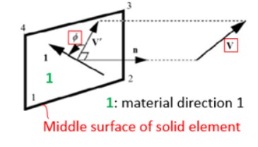
Рисунок 256:

• Толщина и положение слоя

Для толщины и положения твердого элемента, определяемых сеткой элемента.

• Композитный материал, используемый для слоя

  ◦ С опцией mat_IDi можно использовать разные типы материалов для каждого слоя

  ◦ Композитный материал LAW12, LAW14 и LAW25 можно использовать с этим свойством

  ◦ Модель отказа /FAIL/HASHIN, /FAIL/PUCK и /FAIL/LAD_DAMA с этими законами композитного материала также учитываются

  ◦ Материал, указанный в соответствующей карте /PART, используется только для временного шага и расчета жесткости интерфейса

  ◦ Для LAW25 предполагается, что (для твердых тел и толстых оболочек) материал является упругим в поперечном направлении (направление материала 2 и v 1), и в таких случаях необходимо указать значение E33

  Дополнительную информацию см. в разделе «Композитный материал и Разрушение композита».

См. также

/DRAPE (Starter)

Свойства и элементы (FAQ)

Композитная модель отказа

В PRADIOS для описания разрушения композитных материалов могут использоваться следующие модели разрушения композитных материалов. - /FAIL/HASHIN

• /FAIL/PUCK

• /FAIL/LAD_DAMA

• /FAIL/CHANG

16. Л. Горнет, «Прогнозирование повреждений композитных конструкций методом конечных элементов»

Композитный материал состоит из двух разных материалов (матрицы и армирующего волокна). Каждый материал имеет разное поведение при отказе. В PRADIOS можно использовать разные модели отказов для матрицы и волокна в одном композитном элементе (для элементов со свойством TYPE11, TYPE16, TYPE17, TYPE51, PCOMPP или TYPE22). Например, вы можете использовать /FAIL/HASHIN для отказа волокна, /FAIL/PUCK для отказа матрицы и /FAIL/LAD_DAMA для расслоения между слоями или пластами (если для композита определено более одного слоя или пласта).

Помимо вышеперечисленных типичных моделей разрушения композитов, /FAIL/FLD (используется для изотропных хрупких композитных материалов в слоях (пластинах), как в стекле), /FAIL/ENERGY, /FAIL/TBUTCHER и /FAIL/TENSSTRAIN также могут использоваться для описания разрушения композитных слоев (пластин).

/FAIL/HASHIN

При отказе HASHIN рассматриваются два основных режима отказа.

• Режим волокна: композит разрушается из-за разрыва волокна при растяжении или изгиба волокна при сжатии. Таким образом, в /FAIL/HASHIN режим растяжения/сдвига волокна, режим сжатия волокна и режим раздавливания являются режимами волокна. Если

направление 1 является направлением волокна, то плоскость 23 является преобладающей плоскостью отказа для режима волокна.

• Режим матрицы: композит разрушается из-за растрескивания матрицы от волокна.

Режим матрицы разрушения (или режим матрицы разрушения сдвига) и режим расслоения являются режимами матрицы. Плоскость отказа для режима матрицы параллельна волокну, и напряжение \(\sigma\) не будет рассматриваться в этом режиме.

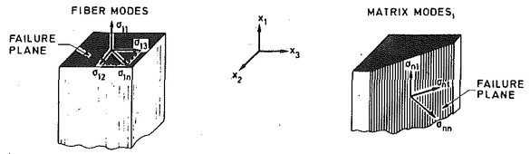
width

6.22864in

height

2.02058in

Рисунок 257: Моды волокон и моды матрицы для однонаправленной модели пластины

Волокна в однонаправленной модели пластины ¹⁷ находятся только в одном направлении, а в модели тканевой пластины — в двух направлениях.

	Однонаправленный Модель ламины	Ткань Ламина модель
Повреждать критерии	Если*D*=1, тогда неудача. Если 0 \(\leq D<1\), D тогда неудача. With \(D=Max(F_{1}, F_{2},F_{3},F_{4})\)	Если*D*=1, тогда неудача. Если 0 \(\leq D<1\), D тогда неудача. With \(D=Max(F_{1}, F_{2},F_{3},F_{4})\)
Растяжение/ сдвиг fiber волокно
Сжатие режим оптоволокна
Режим раздавли- вания
сдвиг отказ matrix режим
отказ матричный режим
Расслаивание режим

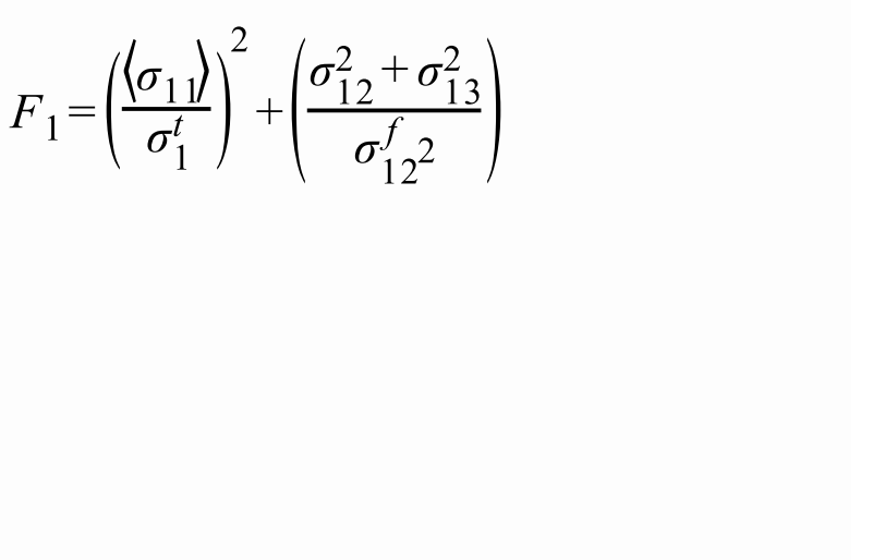
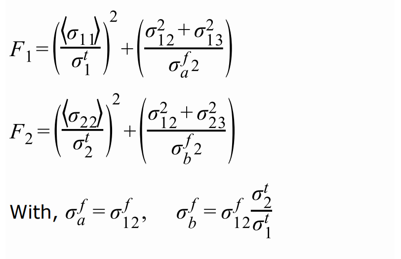
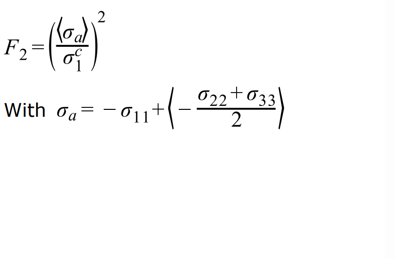
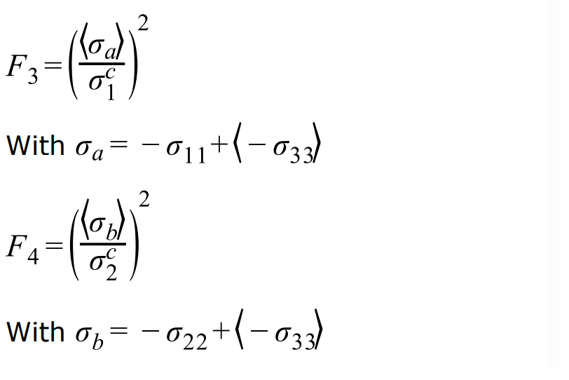
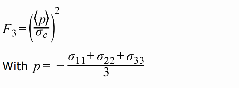
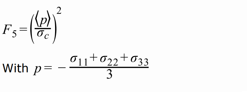
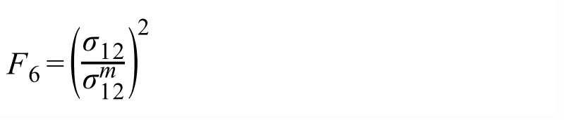
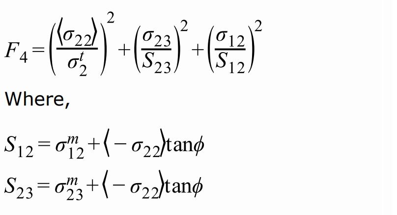
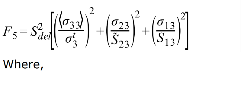
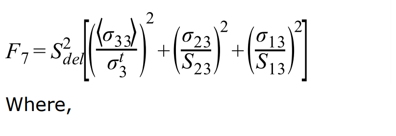
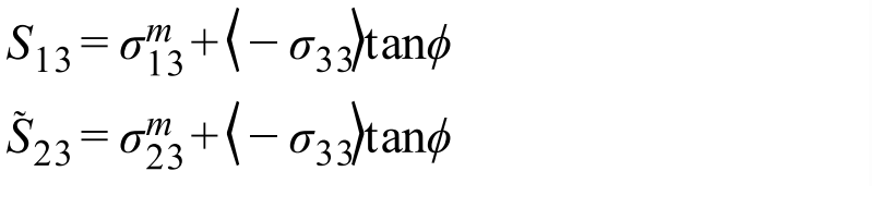
Примечание:\(\left\langle a\right\rangle=\begin{cases}a\ if\ a>0\\ 0\ if\ a<0\end{cases}\)

В /FAIL/HASHIN прочность материала \(\sigma_{1}^{t},\sigma_{2}^{t},\sigma_{3}^{t},\sigma_{1}^{c},\sigma_{2}^{c}\) выводится из испытания на растяжение/сжатие для композита.

Прочность на раздавливание \(\sigma_{c}\) и прочность на сдвиг волокна \(\sigma_{12}^{f}\) могут быть получены из квазистатического испытания на сдвиг ударом (QS-PST). [22] Прочность на раздавливание \(\sigma_{c}\) из отношения пролета к пуансону (SPR) = 0 и прочность на сдвиг волокна \(\sigma_{12}^{f}\) из SPR=1,1.

\(\phi\) — угол трения Кулона. Замечено, что прочность композита на сдвиг выше, если композит также находится под сжатием (а не под растяжением). Это связано с трением между матрицей и волокном.

Предполагается, что прочность на сдвиг пропорциональна напряжению сжатия и вычисляется как:

\[S_{12}=\sigma_{12}^{m}+tan \phi\left\langle-\sigma_{22}\right\rangle \tag{194}\]

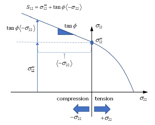
Рисунок 258:

Угол функции \(\phi\) может быть подобран с помощью теста сжатия вне оси с различными углами \(\sigma\) (например, 30 ^◦ , 45 ^◦ , 60 ^◦ , …). .. image:: vertopal_75794439f47d439ba01f734ac3f4dcc1/media/ima–ge142.jpg

width

4.74208in

height

2.16686in

Рисунок 259:

\(\sigma_{12}^{m},\sigma_{13}^{m},\sigma_{23}^{m}\) можно получить из теста на сдвиг матрицы в трех направлениях.

\(S_{del}\) — масштабный коэффициент для критериев расслоения. Он может быть подобран с экспериментальными данными по композитному расслоению, чтобы сбой расслоения коррелировал с площадью повреждения в эксперименте.

/FAIL/PUCK

При разрушении шайбы рассматриваются два типа разрушения.

• Разрушение волокна: композит разрушается из-за того, что волокно достигает предела прочности на растяжение или сжатие.

• Межволоконное разрушение (IFF): композит разрушается из-за растрескивания матрицы волокна.

Повреждать критерии	Если D =1, потом неудача. Если f \(0\leq D<1 D\), потом неудача. с \(D=Max\big{(}e_{f}(tensile),e_{f}(compression), e_{f}(ModeA),e_{f}(modeB),e_{f}(ModeC)\big{)}\)
Фракция волокна отказ	Режим разрушения волокна при растяжении: \(\sigma_{11}>0\) \(e_{f}(tensile)=\frac{\sigma_{11}}{\sigma}_ {1}^{t}\)
	Режим разрушения компрессионного волокна \(\sigma_{11}>0\) \(e_{f}(compression)=\frac{|\sigma_{11}|} {\sigma_{1}^{c}}\)
Межволоконный режим (IFF) 18	Mode A, if \(\sigma_{22}>0\) Рис. 260: \(e_{f}(ModeA)=\frac{1}{\sigma_{12}}\big{[} \sqrt{\big{(}\frac{\sigma_{12}}{\sigma_{2}^{t}} \big{)}^{2}\sigma_{22}2+\sigma_{12}2}+p_{12}^{+} \sigma_{22}\big{]}\)
	Mode C, if \(\sigma_{22}<0\) Рис. 261: \(e_{f}(ModeС)=\big{[}\big{(}\frac{\sigma_{12}} {2(1+p_{22})\sigma_{12}}\big{)}^{2}+\big{(}\frac {\sigma_{22}}{\sigma_{2}^{c}}\big{)}^{2}\big{]} \big{(}\frac{\sigma_{2}^{c}}{-\sigma_{22}}\big{)}\)
	Mode B: Рис. 262: \(e_{f}(ModeB)=\frac{1}{\sigma_{12}}\big{(} \sqrt{\sigma_{12}^{2}+\big{(}p_{12}\sigma_{22} \big{)}^{2}}+p_{12}\sigma_{22}\big{)}\)

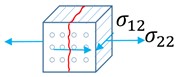
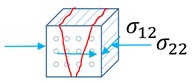
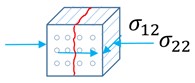
При межволоконном разрушении режим A показывает разрушение при растяжении в поперечном направлении волокон (90 градусов к направлению волокон), и в этом случае сдвиговая нагрузка может снизить предел разрушения.

Если при сжатии в поперечном направлении волокон, сначала увеличение сжатия увеличит композитную сдвиговую нагрузку (режим B). Если сжатие продолжает увеличиваться, то сдвиговая нагрузка уменьшится (режим C).

Входные параметры

Рисунок 263: Кривая разрушения IFF в \(\sigma_{22}-\sigma_{12}\) плоскости

Для \(p_{12}^{+},p_{12}^{-},p_{22}^{-}\) параметров ¹⁹. Для композита из углеродного волокна используйте \(p_{12}^{+}=0,35, p_{12}^{-}=0,3, p_{22}^{-}=0,2\), а для стекловолоконного композита используйте \(p_{12}^{+}=0,3, p_{12}^{-}=0,25, p_{22}^{-}=0,2\).

/FAIL/LAD_DAMA

/FAIL/LAD_DAMA используется для описания расслоения между композитными слоями (распространение повреждений в матрице). Предположим, что слои соединены через виртуальный интерфейс (контакт).

Рисунок 263: Кривая разрушения IFF в \(\sigma_{22}-\sigma_{12}\) плоскости

Для \(p_{12}^{+},p_{12}^{-},p_{22}^{-}\) параметров ¹⁹. Для композита из углеродного волокна используйте \(p_{12}^{+}=0,35, p_{12}^{-}=0,3, p_{22}^{-}=0,2\), а для стекловолоконного композита используйте \(p_{12}^{+}=0,3, p_{12}^{-}=0,25, p_{22}^{-}=0,2\).

/FAIL/LAD_DAMA

/FAIL/LAD_DAMA используется для описания расслоения между композитными слоями (распространение повреждений в матрице). Предположим, что слои соединены через виртуальный интерфейс (контакт).

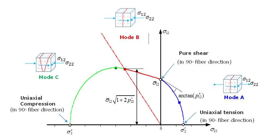
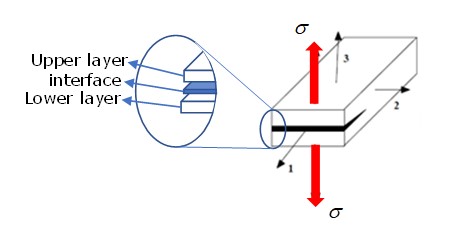
Рисунок 264:

Например, если композит находится под нагрузкой, как показано ниже, тяга \(\sigma\) и смещение в направлении 3

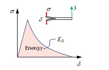
Рисунок 265:

Площадь под кривой растяжения и смещения представляет собой поглощенную энергию расслоения, которая также называется энергией деформации интерфейса повреждения. Разрушение регулируется этой энергией деформации описано ниже, учитывая 3 режима расслоения:

Где, \(\sigma_{3},\sigma_{32},\sigma_{31}\) напряжения, показанные ниже в трех режимах поведения расслоения.

Рисунок 266:

С энергией деформации расслоения \(E_{D}\) термодинамическая сила (контактная сила виртуального интерфейса), также называемая скоростями высвобождения энергии повреждения, может быть рассчитана для этих трех режимов:

• Модель I (образец DCB:sup:21)

\(Y_{d_{3}}=\frac{\partial E_{D}}{\partial d_{3}}\bigg{|}_{\sigma=\text{csf}}=\frac{1}{2}\frac{\left<\sigma_{3}y\right>^{2}}{K_{\frac{3}{3}}(1-d_{3})^{2}}\)

• Model II (ENF specimen:sup:21)

\(Y_{d_{2}}=\frac{\partial E_{D}}{\partial d_{2}}\bigg{|}_{\sigma=\text{csf}}=\frac{1}{2}\frac{\sigma_{3}z^{2}}{K_{\frac{3}{3}}(1-d_{2})^{2}}\)

• Model III

\(Y_{d_{1}}=\frac{\partial E_{D}}{\partial d_{1}}\bigg{|}_{\sigma=\text{csf}}=\frac{1}{2}\frac{\sigma_{3}z^{2}}{K_{\frac{3}{3}}(1-d_{1})^{2}}\)