Где, \(K_{3}, K_{2}, K_{1}\) являются жесткостями виртуального интерфейса, также называемыми межслойной жесткостью. Эти значения могут быть вычислены как: .. math:: K_{3}=frac{2E_{33}}{t}tag{196}

\[K_{2}=\frac{2G_{23}}{t}\]

\[K_{1}=\frac{2G_{13}}{t}\]

Где,

\(t\) Толщина виртуального интерфейса. Можно предположить, что она составляет 1/5 толщины слоя.

\(G_{13}, G_{23}, E_{33}\) Из верхнего или нижнего слоя.

\(d_{i}\) (при \(i\) =1,2,3), переменная повреждения.

Имеет диапазон от 0 до 1. Начинает накапливаться, как только композит достигает \(Y_{0}\).

Пример режима I, во время натяжения в направлении 3, в начале \(d_{3}\) всегда остается 0, пока термодинамическая сила \(Y_{d_{3}}\) не достигнет \(Y_{0}\) (левый рисунок). .. image:: vertopal_7197fe79ded4471fa6ba70c4c62a5530/media/im8age1.jpg

width

5.84217in

height

2.03351in

Рисунок 267:

После достижения \(Y_{0}\) переменная повреждения начинает увеличиваться, и когда она достигает 1, \(d_{3}=1\) (термодинамическая сила \(Y_{d_{3}}\) в этой точке становится критическим повреждением \(Y_{c}\)). Композит можно считать полностью расслоившимся и его можно немедленно удалить или можно уменьшить напряжение. В PRADIOS эта опция используется для моделирования экспоненциального снижения напряжения, и напряжение при \(Y_{c}\) равно \(\sigma_{d}(t_{r})\) (снижение напряжения при повреждении).

Связь с термодинамической силой \(Y_{d_{i}}\) и \(d_{i}\) следующая:

• Если \(d\geq 1\), то принимаем d =1

• Если d <1, то d является функцией Y (закон оценки ущерба):

\[d=w(Y)=\frac{\left\langle{\sqrt{Y}}-{\sqrt{Y_{0}}}\right\rangle}{\sqrt{Y_{c}}-\sqrt{Y_{0}}}\tag{197}\]

\(Y=Y_{d_{3}}+\gamma_{1}Y_{d_{1}}+\gamma_{2}Y_{d_{2}}\text{with}Y_{d_{i}}\left|=\sup Y_{d_{i}}\right|_{\leq t}\)

Здесь \(\gamma_{1},\gamma_{2}\) являются масштабными коэффициентами для рассмотрения двух других режимов расслоения. Это может быть подтверждено экспериментами (тест образца DCB и ENF:sup:21).

В примере режима I \(\gamma_{1},\gamma_{2}\) может быть 0, поскольку это чистое расслоение в направлении 3, и тогда \(Y=Y_{d_{3}}\) соотношение \(Y_{d_{3}}\) и \(d_{3}\) равно:

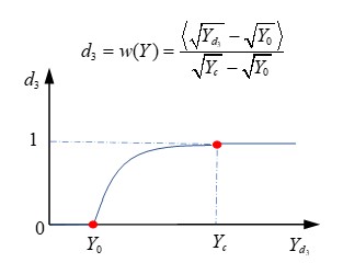
Рисунок 268:

Как быстро будет увеличиваться переменная повреждения? Скорость повреждения \(d\) (также называемая законом оценки повреждения) вычисляется как:

• Если \(d=1\), то \(\dot{d}=\textit{const.}\)

• Если \(d<1\), то \(\dot{d}=\frac{k}{a}\big{[}1-\exp\big{(}-\alpha\big{(}w(Y)-d\big{)}\big{)}\big{]}\)

\(\frac{k}{a}\) - это максимальная скорость повреждения, что означает минимальную продолжительность явления отказа. Его обратная величина, \(\frac{a}{k}\) называется характерным временем, которое можно получить с помощью одномерного испытания на растяжение.

23

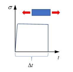
Рисунок 269:

Через растяжение образца с различным напряжением для нахождения минимального времени композитного повреждения \(\Delta \)sigma-Delta t` является вертикальной асимптотой, соответствующей характерному времени \(\frac{a}{k}\).

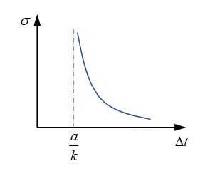
Рисунок 270:

Параметры (a) и (k) управляют законом оценки повреждений. Например, при постоянном параметре (a) (здесь (a=1)) уменьшение значений (k) приводит к более хрупкому разрушению композита.

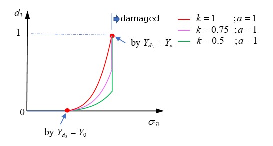
Рисунок 271:

При постоянном параметре (k) (здесь (k=1)) увеличение значений (a) приводит к более хрупкому разрушению композита.

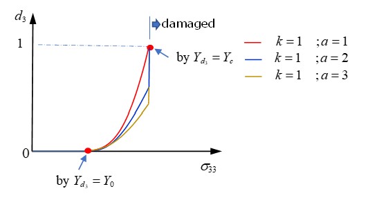
Рисунок 272:

/FAIL/CHANG

При отказе Чанга-Чанга рассматриваются два основных режима отказа.

• Режим волокна: композит выходит из строя из-за разрыва волокна при растяжении или изгиба волокна при сжатии.

• Режим матрицы: композит выходит из строя из-за разрушения матрицы при растяжении или сжатии.

Этот критерий отказа используется только для элементов оболочки.

Повреждение критерий		Если D =1, тогда неудача. Если \(0\leq D<1\) D, тогда никаких неудач. с \(D=Max(e_{f}2,e_{c}2,e_{m} 2,e_{d}2)\).
Волокно поломка	Режим растяжения волокна \(\sigma_{11}>0\)	\(e_{f}2=\big{(}\frac{\sigma_{11}} {\sigma_{1}^{t}}\big{)}^{2}+\beta\big{(} \frac{\sigma_{12}}{\sigma_{12}}\big{)} ^{2}\)
	Режим компрессионного волокна \(\sigma_{11}<0\)	:math:`e_{c}2=big{(}frac{sigma_{11}} {sigma_{1}^{c}}big{)}^{2}`
Матрица трещины	Режим растяжения матрицы \(\sigma_{22}>0\)	\(e_{m}2=\big{(}\frac{\sigma_{11}} {\sigma_{1}^{t}}\big{)}^{2}+\beta\big{(} \frac{\sigma_{12}}{\sigma_{12}}\big{)} ^{2}\)
	Режим компрессионной матрицы \(\sigma_{22}<0\)	:math:`e_{d}2=big{(}frac{sigma_{22}} {2sigma_{12}}big{)}^{2}+big{[}big{(} frac{sigma_{2}^{c}}{2sigma_{12}} big{)}^{2}-1big{]}frac{sigma_{22}} {sigma_{2}^{c}}+big{(}frac {sigma_{12}}{sigma_{12}}big{)}^{2}`

Где,

направление 1 Направление волокон.

\(\sigma_{1}^{t},\sigma_{1}^{c}\) Прочность волокон на растяжение/сжатие.

\(\sigma_{2}^{t},\sigma_{2}^{c}\) Прочность матрицы. Растягивающая или сжимающая нагрузка в направлении 2 (поперечном направлению 1).

\(\sigma_{12}\) Прочность на сдвиг в плоскости композитного слоя.

\(\beta\) Масштабный коэффициент сдвига, который можно определить экспериментально.

Уменьшение напряжения при повреждении

После достижения критерия повреждения:

• HASHIN:

\(D=Max(F_{1},F_{2},F_{3},F_{4})\geq 1\)

• PUCK:

\(D=Max(e_{f}(tensile),e_{f}(compression),e_{f}(ModeA),e_{f}(ModeB),e_{f}(ModeC))\geq 1\) • LAD_DAMA:

\(d\geq 1\)

• CHANG:

\(D=Max(e_{f}2,e_{c}2,e_{m}2,e_{d}2)\geq 1\)

Напряжения начинают уменьшаться и уменьшаются постепенно с использованием экспоненциальной функции, чтобы избежать числовых нестабильностей.

\[\sigma(t)=\sigma_{d}(t_{r})\cdot\text{f}(t)\tag{198}\]

\(=\sigma_{d}(t_{r})\cdot\exp\Big{(}-\frac{t-t_{r}}{t_{\max}}\Big{)}\)

с, \(t\geq t_{r}\)

Опция \(\tau_{\max}\) контролирует, насколько постепенно уменьшается напряжение при повреждении.

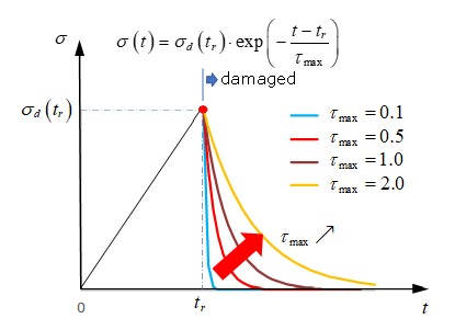
Рисунок 273:

Где,

\(\sigma_{d}(t_{r})\) Компоненты напряжения при достижении повреждения \(D\geq 1\).

\(t_{r}\) Время \(\sigma_{d}(t_{r})\).

\(t_{max}\) Время динамической релаксации.

Чем выше значение \(t_{max}\), тем медленнее снижается напряжение при повреждении.

Обычно для прогнозирования разрушения ламинированных композитов при динамической нагрузке требуется 10~20 временных шагов моделирования.

17. Hashin, Z., “Failure Criteria for Unidirectional Fiber Composites,” Journal of Applied Mechanics, Vol. 47, 1980, pp. 329-334.

18. 1. Puck, J. Kopp, and M. Knops., “Failure analysis of FRP laminates by means of physically based phenomenological models”. Composites Science Technology, 62. pp. 1633-1662. 2002.

19. 1. Puck, J. Kopp, and M. Knops. “Guidelines for the determination of the parameters in Puck’s action plane strength criterion”. Composites Science Technology 62. pp. 371-378. 2002.

20. 12. Gornet, “Finite Element Damage Prediction of Composite Structures”.

21. Ladevèze, P., Allix, O., Douchin, B., Lévêque, D., “A Computational Method for damage Intensity Prediction in a Laminated Composite Structure”, Computational mechanics—New Trends and Applications In: Idelsohn, S., Oñate E., and Dvorkin E., (eds.) CIMNE, Barcelona, Spain (1998).

22. Gama B.A., Gillespie J.W., Punch Shear Behavior of Composites at Low and High Rates[M]// Fracture of Nano and Engineering Materials and Structures. Springer Netherlands, 2006.

23. Allix, O. & Deü, Jean-François. (1997). Delay-damage modeling for fracture prediction of laminated composites under dynamic loading. Engineering Transactions. 45. 29-46.

Соединения

Точечная сварка (болтовое или клеевое соединение)

Существует три различных способа моделирования точечных сварных швов:

• Узловое соединение

• Пружинное (/PROP/TYPE13) соединение

• Твердое соединение

Пружинное (/PROP/TYPE13) соединение и твердое соединение также могут использоваться для моделирования болтового или клеевого соединения (клея).

Узловое соединение

Единый интерфейс TYPE2 с первой поверхностью в качестве основной стороны и некоторыми узлами со второй поверхности в качестве вторичных узлов: При таком решении сетка основной поверхности может быть независимой от места точечной сварки. Проблемы песочных часов исчезают на основной поверхности. На второй оболочке поверхностная сетка должна учитывать место точечной сварки, и проблема песочных часов останется. Основная проблема с этим подходом к моделированию заключается в недеформируемости соединения и его бесконечной прочности.

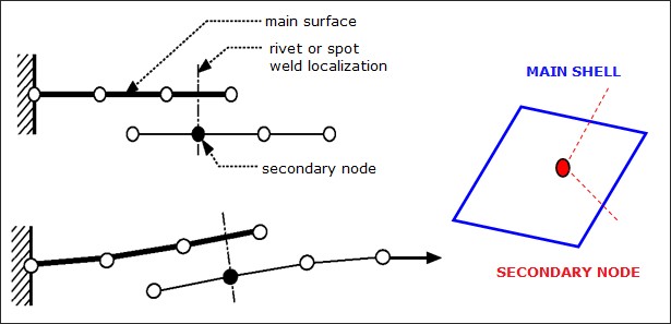
Рисунок 274: Пример соединения между 2 поверхностями оболочки

Пружинное (/PROP/TYPE13) соединение

Два связанных интерфейса и пружина: использование двух связанных интерфейсов обеспечит полное симметричное решение, позволяющее создать свободную сетку на двух поверхностях и избежать песочных часов. Точечный шов моделируется пружинным элементом балочного типа. Пружинный элемент использует независимые узлы, не связанные с элементами оболочки. Один из двух узлов расположен на первой поверхности (или рядом с ней, нет необходимости расположения точно на поверхности оболочки), а второй узел расположен на второй поверхности. Один связанный интерфейс соединяет один пружинный узел с первой поверхностью, а второй связанный интерфейс делает то же самое для второго узла на второй поверхности.

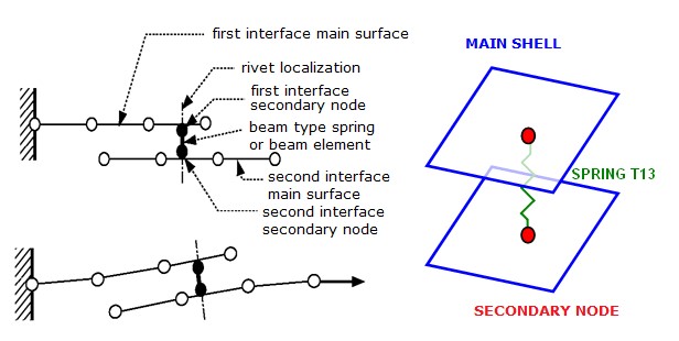
Рисунок 275: Моделирование точечной сварки

Создание точечной сварки с использованием этого метода является хорошим альтернативным решением при таком подходе место соединения не зависит от сетки оболочки. Это точнее, чем приведенное выше моделирование узлового соединения поскольку свойства точечной сварки вводятся непосредственно для пружины TYPE13.

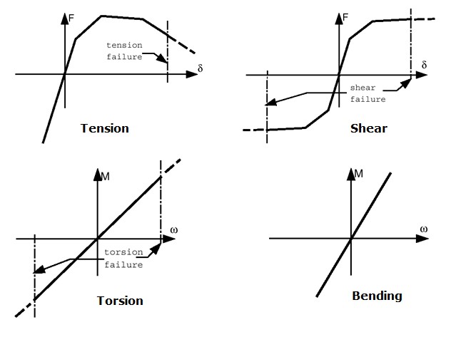
Рисунок 276: Пружина TYPE13 — типичный ввод для точечной сварки

Более того, существует два разных способа моделирования разрыва точечной сварки:

1. Использовать критерии отказа, доступные для пружины TYPE13. Более подробную информацию см. в комментариях к критериям отказа в /PROP/TYPE13 (SPR_BEAM).

2. Использовать \(Spot_{flag}\) = 20, 21 или 22 в связанном контакте (связанный контакт (/INTER/TYPE2)).

   Примечание: Методика моделирования пружин TYPE13 для точечной сварки

   может также использоваться для других видов соединений, таких как линии сварки, подгибка, клей и болты. Для моделирования болтов использование связанного интерфейса не обязательно, так как узлы оболочки можно поместить непосредственно в жесткие тела.

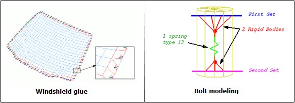
Рисунок 277: Примеры моделирования с использованием клея и болтов

Примечание: При связанном интерфейсе масса вторичного узла

передается в основные узлы, если \(Spot_{flag}\) установлен на 1. Инерция вторичного узла равномерно распределяется по основным узлам путем добавления массы, так что индуцированная инерция (в центре основной поверхности) равна инерции вторичного узла. Если основная поверхность является идеальным квадратом, добавленная масса вычисляется как:

\(l_{s}=4\Delta m\cdot L^{2}\)

\(\Delta m\) : добавленная масса

\(L\) : расстояние между главным узлом и центром

\(l_{s}\) : инерция вторичного узла

Пока инерция вторичного узла реалистична, добавленная масса будет очень мала. Большая добавленная масса наблюдается, если вторичный узел находится слишком далеко от основной поверхности. Идеальным является расположение вторичного узла на плоскости основной поверхности, прямо в ее центре. Если это не так, вторичный узел имеет инерцию в центре поверхности оболочки:

\(l_{s}=m_{s}\cdot L_{s}2\)

\(m_{s}\) Масса вторичного узла

\(L_{s}\) Расстояние между вторичным узлом и центром

\(l_{s}\) Iнервия вторичного узла

Следовательно, новая добавленная масса устанавливается для основных узлов, так что инерция (из-за этой новой добавленной массы) равна инерции, из-за смещения вторичного узла.

\[4\Delta m\cdot L^{2}=m_{s}\cdot L_{s2}\tag{199}\]

Если \(Spot_{flag} =0\) , то нет никакой добавленной массы, так как инерция вторичного узла вместо этого передается как инерция основному узлу. Слишком большая добавленная инерция серьезно снизит точность.

См. также

RD-E: 4802 Твердая и пружинная точечная сварка в Crash Box

Твердая точечная сварка

Использует 8-узловой элемент кирпича (с /PROP/TYPE43) и /MAT/LAW59``+ ``/FAIL/CONNECT (или /MAT/LAW83``+ ``/FAIL/SNCONNECT) для моделирования сплошных точечных сварных швов, что может обеспечить более точные результаты.

Твердый элемент и свойство

Элемент кирпича использует /PROP/TYPE43 и имеет 4 точки интегрирования на плоскости сдвига, которая находится между плоскостью (1, 2, 3, 4) и плоскостью (5, 6, 7, 8). Есть одна точка интегрирования в нормальном направлении t.

Этот тип элемента не имеет самого временного шага, и его устойчивость обеспечивается его узловыми соединениями. Это означает, что толщина точечной сварки может быть очень малой. Эта характеристика очень полезна для моделирования клея.

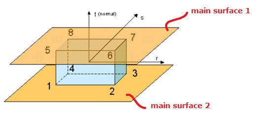
Рисунок 278: .. image:: vertopal_7197fe79ded4471fa6ba70c4c62a5530/media/image16.jpg

width

3.82533in

height

1.75849in

Рисунок 279:

Соединение с листом оболочки (Shell Sheet)

/INTER/TYPE2 может использоваться для соединения сплошных точечных сварных швов с двумя (верхней и нижней) основными поверхностями. Узлы плоскости (1,2,3,4) привязаны к одной оболочке, и узлы плоскости (5,6,7,8) привязаны к другой оболочке. Не допускается, чтобы какая-либо другая плоскость (например, плоскость (1,4,8,5)) была привязана к оболочке.

Модель материала и отказа

Сплошные точечные сварные швы в PRADIOS могут быть смоделированы с помощью /MAT/LAW59``+ ``/FAIL/CONNECT (или /MAT/LAW83``+ ``/FAIL/SNCONNECT). Эта модель материала должна быть проверена с четырьмя случаями нагрузки точечной сварки испытаний.

• Испытание на сдвиг (угол нагрузки и верхняя поверхность точечной сварки составляет 0 градусов ниже названного испытания на 0 градусов)

• Нормальное испытание на растяжение (испытание 90 градусов),

• Сдвиг и нормальное комбинированное испытание (например, испытание 30 градусов, испытание 45 градусов или испытание 90 градусов)

• Испытание на момент (испытание на отслаивание)

Модуль упругости

Жесткость точечной сварки в разных испытаниях различна. В нормальном испытании она ниже, чем в испытании на сдвиг, из-за деформации верхнего и нижнего листов. Поэтому обычно измеренная жесткость берется из истинной кривой напряжения от смещения испытания на сдвиг.

/MAT/LAW59+/FAIL/CONNECT

• Кривая текучести материала:

  В LAW59 запрашиваются кривые текучести материала точечной сварки в нормальном направлении и в направлении сдвига. Кривая текучести (\(Y\_fct\_ID_{N}\)) в нормальном направлении может быть определена из нормального испытания на растяжение (испытание под углом 90 градусов), а кривая текучести (\(Y\_fct\_ID_{T}\)) в направлении сдвига может быть определена из испытания на сдвиг (испытание под углом 0 градусов).

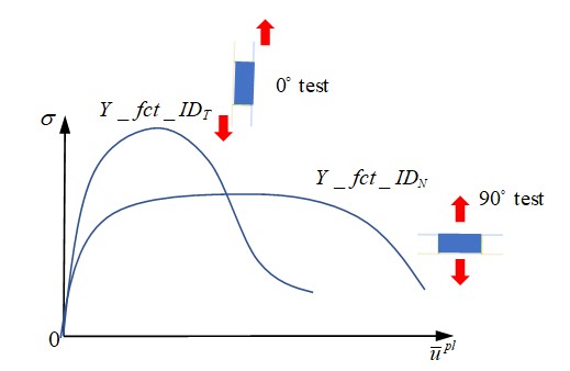
Рисунок 280:

В этом случае максимальное напряжение также описывается внутри кривых. Учитывая опорную скорость смещения \(SR_{ref}\) входной кривой текучести, PRADIOS будет учитывать эффект скорости смещения относительно этой опорной скорости смещения.

• Разрушение точечной сварки:

  Повреждение и отказ сплошной точечной сварки можно рассматривать с помощью /FAIL/CONNECT. Критерии смещения и/или энергетические критерии могут использоваться для описания отказа точечной сварки. ◦ Для критериев смещения отказ происходит, когда достигается нормальное смещение или сдвиговое смещение в соответствии с двумя альтернативными типами поведения:

  ∙ Несвязанный отказ (\(I_{fail} =0\): однонаправленный отказ)

\[\overline{n}_{i}\cdot\mathrm{f}(\overline{u})>\overline{n}_{maxi}\tag{200}\]

with i = 33 для нормального направления и i = 13 или 23 для касательных направлений.

В нормальном испытании на растяжение (испытание на 90 градусов) элемент выходит из строя, как только достигается заданное пользователем максимальное смещение \(\overline{n}_{max N}\).

В испытании на сдвиг и растяжение (испытание на 0 градусов) элемент выходит из строя, как только достигается заданное пользователем максимальное смещение \(\overline{n}_{max T}\).

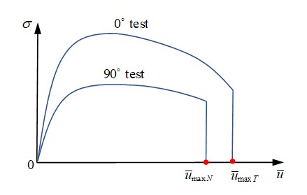
Рисунок 281:

В комбинированном режиме испытания (например, 30-градусный тест или 60-градусный тест) разрушение в сплошном точечном шве не учитывает сдвиг и нормальный эффект комбинированного напряжения. Разрушение в каждом направлении рассматривается отдельно. Элемент разрушается, как только любое из этих двух напряжений достигает соответствующего максимального смещения. Чтобы учесть комбинированные напряжения, вместо этого установите \(I_{fail} =1\), и тогда будет рассмотрен эффект комбинированного напряжения.

∙ Связанный отказ (\(I_{fail} =1\): многонаправленный отказ)

\[\left\|\frac{\overline{n}_{N}}{\overline{n}_{\max N}}\cdot\alpha_{N}\cdot \mathrm{f}_{N}(\overline{u}_{N})\right\|^{\exp_{N}}+\left\|\frac{\overline{n}_{T}}{\overline{n}_{\max_{T}}}\cdot\alpha_{T}\cdot\mathrm{f}_{T}(\overline{u}_{T})\right\|^{\exp_{T}}>1 \tag{201}\]

При \(I_{fail} =1\), в комбинированном режиме испытания элемент выходит из строя до достижения максимального напряжения или того, что ближе к реальности. Для описания поверхности разрушения кривой вам необходимо как минимум 4 различных комбинированных испытания для соответствия параметрам \(a_{N},a_{T},\exp_{N},\exp_{T}.\)

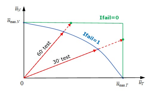
Рисунок 282: Поверхность разрушения

◦ Для энергетических критериев отказ происходит, когда достигается внутренняя энергия в нормальном направлении или внутренняя энергия в направлении сдвига, что соответствует максимальной внутренней энергии

\(EN_{max},ET_{max}.\)

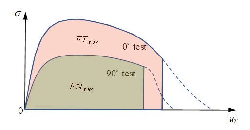
Рисунок 283:

В комбинированном режиме испытания отказ элемента также рассматривается с учетом многонаправленного воздействия на внутреннюю энергию. Если введены внутренняя энергия в нормальном направлении и в направлении сдвига, элемент терпит неудачу, если удовлетворяется через:

\[\left(\frac{En}{EN_{\text{max}}}\right)^{N_{n}}+\left(\frac{Et}{ET_{\text{max}}}\right)^{N_{t}}\geq 1\tag{202}\]

Если ввести только полную внутреннюю энергию \(EI_{max,}\), элемент терпит неудачу, если удовлетворяется через:

\[\frac{E(t)}{EI_{\text{max}}}\geq 1\tag{203}\]

Если введены оба \(EI_{max}\) и \(EN_{max,}ET_{max}\), элемент терпит неудачу, в зависимости от того, какой из этих двух критериев будет достигнут первым. Могут быть определены как критерии смещения, так и энергетические критерии. Элемент выходит из строя из-за того, какой критерий достигается первым. Удаление элемента происходит, когда одна точка интегрирования достигает критериев отказа, если \(I_{solid} =1\) или когда все точки интегрирования достигают критериев отказа, если \(I_{solid} =2\).

• Размягчение точечной сварки:

После достижения критерия отказа (критерия смещения или критерия энергии) напряжение снижается до 0 напрямую или может постепенно управляться параметрами \(T_{max}\) и \(N_{soft}\) с:

\[\sigma=\sigma_{f}\left(1-\frac{D}{T_{\text{max}}}\right)^{N_{soft}}\tag{204}\]

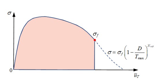
Рисунок 284:

Рисунок 285 показывает влияние различных \(T_{max}\) на поведение снижения напряжения.

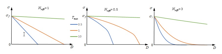
Рисунок 285:

/MAT/LAW83+/FAIL/SNCONNECT

• Кривая текучести материала:

В LAW83 кривая материала точечной сварки может быть введена с помощью \(fct\_ID_{1}\). Там, где во вводе LAW59 требуются две кривые текучести для нормального направления и направления сдвига, LAW83 использует только одну кривую. Эта кривая должна брать кривую текучести из испытания на сдвиг. Кроме того, кривая текучести \(fct\_ID_{1}\) для LAW83 не определяется как истинное напряжение против пластического смещения (как в LAW59), а должна быть нормализованной кривой напряжения против пластического смещения. Предел текучести нормализуется максимальным напряжением, которое вводится как параметры \(R_{N,}R_{S}\) в LAW83

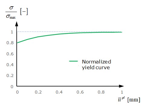
Рисунок 286:

Кривая текучести отличается из-за различных комбинаций нормального напряжения и напряжения сдвига в точечной сварке. Это можно описать с помощью параметра \(\beta\) в LAW83 (он не учитывается в LAW59). Нормализованный предел текучести в LAW83 равен:

\[\sigma_{y}=\left[\left(\frac{\sigma_{n}}{R_{N}\cdot\mathrm{f}_{N}(1-\alpha\cdot\mathrm{sym})}\right)^{\beta}+\left(\frac{\sigma_{s}}{R_{S}\cdot\mathrm{f}_{S}}\right)^{\beta}\right]^{\frac{1}{\beta}}\tag{205}\]

В случаях, когда эффект момента не учитывается, нормализованный предел текучести в LAW83 равен:

\[\sigma_{y}=\left[\left(\frac{\sigma_{n}}{R_{N}\cdot\mathrm{f}_{N}}\right)^{\beta}+\left(\frac{\sigma_{s}}{R_{S}\cdot\mathrm{f}_{S}}\right)^{\beta}\right]^{\frac{1}{\beta}}\tag{206}\]

На рисунке 287 показана разница нормализованного максимального напряжения в комбинированных испытаниях между LAW83 и LAW59.

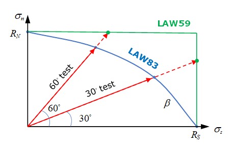
Рисунок 287:

На рисунке 288 показано влияние изменения \(\beta\) на нормализованное максимальное напряжение в комбинированных тестах с использованием LAW83.

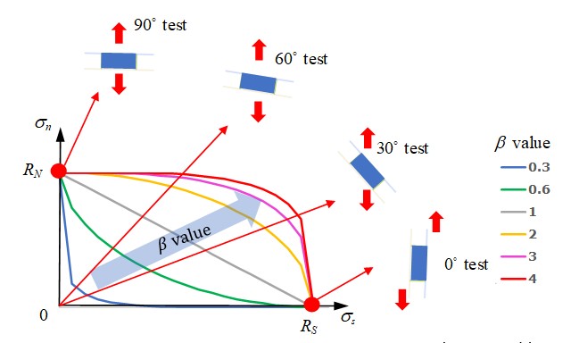
Рисунок 288:

Параметр a используется для описания эффекта момента в точечной сварке.

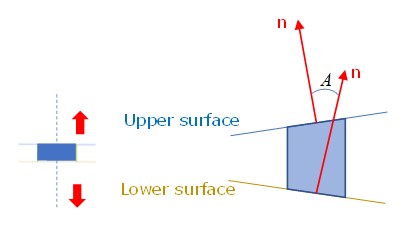
Рисунок 289: Испытание на нецентральное растяжение (испытание на отрыв)

Используйте a для уменьшения максимального напряжения испытания на отрыв. — это синус угла между верхней и нижней поверхностью точечной сварки. Он изменяется во время деформации точечной сварки и находится в диапазоне [-1,1]. Параметр можно подогнать с помощью простой модели FEM для соответствия реальным экспериментальным данным. ²⁴

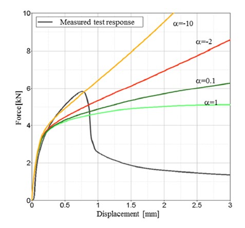
Рисунок 290: Различные эффекты при испытании на отрыв при силе в зависимости от смещения

Влияние скорости смещения на кривую текучести материала также можно рассмотреть с помощью входных данных кривой \(fct\_ID_{N}\) и \(fct\_ID_{S}\).

• Повреждение и отказ материала:

Для отказа точечной сварки можно использовать /FAIL/SNCONNECT. В этой модели отказа необходимы пластические смещения (как в нормальном, так и в направлении сдвига) начала повреждения и отказа.

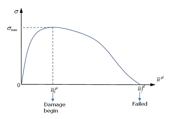
Рисунок 291:

Для комбинированного режима испытания, аналогичного максимальному напряжению в LAW83, необходимо описать пластическое смещение в начале повреждения и описать пластическое смещение при отказе.

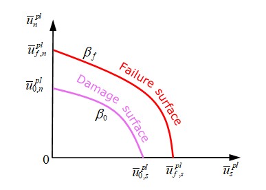
Рисунок 292:

Для точечной сварки с моментом (испытание на отслаивание), аналогично максимальному напряжению в LAW83, необходимо \(\beta_{0}\) для описания пластического смещения в начале повреждения во время испытания на отслаивание и \(\beta_{f}\) для описания пластического смещения при отказе испытания на отслаивание.

Таблица 20: Общие возможности двух подходов к моделированию точечной сварки

		/MAT/LAW59 +/FAIL/CONNECT		/MAT/LAW 83+/FAIL/ SNCONNECT
Кривая роста		Две кривые роста (в нормальным и сдвигом направлениями)		Одна нормализ-нная кривые текучести с максимальным напряжением \(R_{N,} R_{S}\)
Максимум стресс в комбинированный тест режима		Нормальный и сдвигать эффект в комбинированный тест не обдуманный.		Используйте a для учитывать нормальный и сдвиг эффект в комбиниро- ванный режимные испытания.

| | испытания. |

ванный | с :math:`a_{T},a_{N}, | |

| тест режима | exp_{T},exp_{N}` в |Controlled with|

| | смещению |:math:`beta |

| | |_{0},\beta_{f}`|

| | критерии и с :math:`N| |

| | _{n},N_{t}` в энергии | |

| | критерии. | |

| Момент | Нет | Контролируемый|

| эффект | управление на входе | с |

| (тест на | | :math:`a_{0}, |

| пилинг) | | a_{f}` |

| Смягчение | С | С ссылкой |

| | (напряжение | |

| | кривая уменьшается) | к повреждению |

| | | смещению |

| | | |

| | | и отказу |

| | | смещению |

| | | (напряжение |

| | | линейное |

| | | уменьшение) |

| | | |

24. Pasligh, N., Schilling, R., and Bulla, M., “Modeling of Rivets Using a Cohesive Approach for Crash Simulation of Vehicles in PRADIOS,” SAE Int. J. Trans. Safety 5(2):2017, doi:10.4271/2017-01-1472

Моделирование болтов для столкновений

Существуют различные способы моделирования болтовых соединений и более подробная точность модели результатов:

• Жесткий болт

• Жесткий болт с пружиной (и предварительным натяжением)

• Деформируемый болт с пружиной и предварительным натяжением

• Деформируемый болт с начальным напряжением

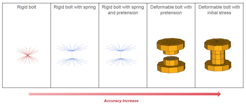
Рисунок 293: Методы моделирования болтов

Жесткий болт

Использование одного жесткого тела (/RBODY), соединенного с деталями, к которым прикреплен болт, является самым простым методом. Хотя этот метод очень стабилен и прост в моделировании, вы не можете учитывать предварительное натяжение, упругопластичность и поведение при разрыве для болта, а выходная сила отсутствует, и моделировать прохождение головки болта через отверстие невозможно.

Рисунок 294: Метод моделирования жесткого болта

Примечание: Основной узел должен быть свободным.

Жесткий болт с пружиной (и предварительным натяжением)

Используйте два жестких тела (/RBODY), соединенных с каждым набором деталей, которые связаны с болтом, а затем установите один пружинный элемент (/PROP/SPR_BEAM) между обоими жесткими телами. С помощью этого метода можно описать упругопластическое поведение разрыва в любом направлении, а силу, проходящую через болт (нормальная сила, усилие сдвига, моменты), можно вывести, используя /TH/SPRING. Этот метод часто используется при анализе автомобильных столкновений, но он имеет ограниченные возможности для моделирования предварительного натяжения.

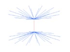
Рисунок 295: Жесткий болт с пружиной

Примечание:

1. Основной узел должен быть свободным.

2. TПружинный элемент прикреплен к жестким телам в качестве вторичного узла.

Для описания предварительного натяжения с помощью этого метода необходимо добавить еще два пружинных элемента (/PROP/SPR_PRE и /PROP/SPR_BEAM). /IMPDISP или /CLOAD можно использовать для имитации предварительной нагрузки. Состояние автобаланса рассчитывается PRADIOS.

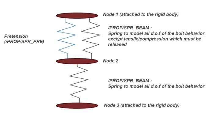
Рисунок 296: Моделирование предварительного натяжения с помощью пружин

Деформируемый болт с пружиной и предварительным натяжением

Сетчатый болт с твердыми элементами (/BRICK или любой другой тип твердого элемента) и разрезом посередине. Два твердых тела, соединенных с каждой стороной сетчатого болта и пружинного ряда (две пружины с /PROP/SPR_BEAM и одна пружина с /PROP/SPR_PRE), как указано выше, между твердыми телами используются для описания предварительного натяжения. С помощью этой более подробной модели головка болта, проходящая через отверстие, может быть рассмотрена в моделировании.

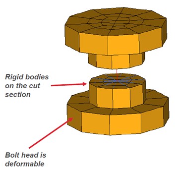
Рисунок 296: Моделирование предварительного натяжения с помощью пружин

Деформируемый болт с пружиной и предварительным натяжением

Сетчатый болт с твердыми элементами (/BRICK или любой другой тип твердого элемента) и разрезом посередине. Два твердых тела, соединенных с каждой стороной сетчатого болта и пружинного ряда (две пружины с /PROP/SPR_BEAM и одна пружина с /PROP/SPR_PRE), как указано выше, между твердыми телами используются для описания предварительного натяжения. С помощью этой более подробной модели головка болта, проходящая через отверстие, может быть рассмотрена в моделировании.

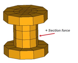
Рисунок 298: Полностью сетчатый деформируемый болт

Примечание:

1. Точность определения разрыва и напряжения зависит от размера ячейки.

2. SСила сжатия в болте необходима для измерения сил, проходящих через отверстие.

Кинематические ограничения

В PRADIOS кинематическое условие — это узловое ограничение, применяемое к набору узлов.

Существует несколько различных типов узловых ограничений:

• Жесткая стена

• Жесткое тело

• Граничные условия

• Связанный интерфейс

• Цилиндрическое соединение

• Жесткое звено

• Соединение зубчатого типа

Численные методы, доступные в PRADIOS, которые применяются к кинематическим условиям:

: Метод штрафа: Жесткие стенки

: Основное вторичное кинематическое условие: Интерфейс TYPE2, жесткое тело

: Локальное кинематическое условие: Жесткое звено, цилиндрическое соединение

: Множитель Лагранжа: Старые и новые интерфейсы, жесткая стена, жесткое тело и т. д.

Жесткое тело (/RBODY)

Жесткое тело определяется набором вторичных узлов и главным узлом. Его можно сравнить с деталью с бесконечной жесткостью. Между вторичными узлами не допускается относительное смещение, а общее движение жесткого тела управляет главным узлом.

Поскольку кинематическое условие применяется к каждому вторичному узлу и для всех направлений, никакие другие узловые ограничения не допускаются. Однако в случае метода множителей Лагранжа решение может быть найдено, если не применяются несовместимые кинематические условия.

Доступны четыре варианта для позиционирования центра тяжести жесткого тела:

Case 1

Центр тяжести вычисляется с учетом массы и координат вторичных и основных узлов. Масса твердого тела представляет собой сумму добавленной массы и массы вторичных узлов.

Case 2

COG вычисляется только с учетом массы и координат вторичных узлов. Масса твердого тела представляет собой сумму добавленной массы и массы вторичных узлов.

Case 3

COG устанавливается в координатах главного узла

Case 4

Масса твердого тела равна сумме добавленной массы и массы вторичного узла. Центр тяжести задается в координатах основного узла. Масса твердого тела равна добавленной массе.

Настоятельно рекомендуется использовать искусственный узел (не являющийся частью элемента) в качестве основного узла, поскольку PRADIOS Starter, скорее всего, переместит основной узел. Основной узел перемещается PRADIOS Starter в центр тяжести; если только флаг ICoG не установлен на 3 или 4. Рекомендуется установить ICoG на 2, чтобы получить наиболее реалистичное поведение; затем центр тяжести вычисляется с учетом только вторичных узлов. Если ICoG установлен на 1, основной узел с собственной массой включается для вычисления центра тяжести.

Если основной узел изначально установлен в центр тяжести, поведение с использованием ICoG = 1 или 2 аналогично.

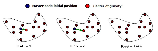
Рисунок 299: Вычисление центра тяжести

В моделировании автокатастрофы в основном используются жесткие тела, и можно выделить три типичных варианта использования жестких тел:

• Жесткое тело, покрывающее часть модели конечных элементов, включая оболочки, твердые тела или другие элементы: в этом случае масса вторичных узлов дает общую массу жесткого тела, и дополнительная масса не требуется. Главный узел может быть расположен где угодно, и он будет перемещен в центр масс. Этот тип жесткого тела экономит большое количество процессорного времени.

• Жесткое тело, представляющее немоделируемый компонент, соединенный с некоторыми структурными узлами: в этом случае для соединения жесткого тела с моделью конечных элементов используется только несколько вторичных узлов. Масса и инерция добавляются, а главный узел располагается в центре масс компонента. Главный узел будет двигаться лишь немного, учитывая массу вторичных узлов. В некоторых случаях фиктивная сетка используется для визуализации жесткого тела или для моделирования контактов, но если фиктивные элементы имеют небольшую массу, предыдущие замечания по-прежнему верны.

• Жесткое тело, используемое для соединения двух или более частей вместе: для этих жестких тел не требуется дополнительная масса, а главный узел может быть расположен где угодно. Для этих жестких тел необходимо использовать сферическую инерцию; поскольку эти жесткие тела обычно очень малы (от 4 до 8 узлов), инерция часто очень мала в одном направлении и очень велика для одного конкретного направления. Это может привести к нестабильности; поэтому, благодаря использованию сферической инерции, инерция будет одинаковой для любого направления.

Активация/Деактивация

Твердые тела можно активировать или деактивировать с помощью /SENSOR или с помощью параметров движка /RBODY/ON или /RBODY/OFF.

Чтобы активировать два твердых тела с помощью главного узла 1 и 2, добавьте следующую опцию в Rootname_0001.rad:

/RBODY/ON

1 2

Все элементы, входящие в состав обоих жестких тел, деактивированы.Все элементы, входящие в состав обоих жестких тел, деактивированы. Чтобы деактивировать одно твердое тело, идентификатор основного узла которого равен 3, добавьте:

/RBODY/OFF

3

Все элементы реактивированы, деформации и напряжения соответствуют значениям, оставшимся со времени предыдущей дезактивации.

Движения твердого тела

Одно из основных применений активации и деактивации твердого тела касается движений опрокидывания, как при моделировании опрокидывания. Во время свободного полета автомобиля деформацией элементов можно пренебречь. Значительную часть времени ЦП можно сэкономить, если всю конструкцию заменить временным жестким телом во время полета. Перед ударом о землю это твердое тело деактивируется и в конечном итоге снова активируется после отскока.

Двигатель

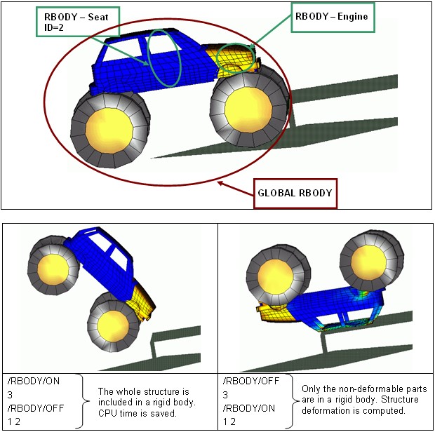
Рисунок 300: Активация - деактивация твердых тел в примере опрокидывания

Начальное статическое равновесие

Другое применение активации и деактивации жесткого тела - для начального статического равновесия, где применяется только сила тяжести. При анализе краш-теста может быть интересно установить весь автомобиль в равновесии над подвеской, а манекен - на сиденье. Для явного анализа требуется много времени, чтобы достичь статического равновесия; следовательно, использование большого твердого тела позволяет быстрее получить решение. Однако в этом случае деформация в автомобиле или манекене под действием силы тяжести игнорируется, и за обоснованностью этого предположения необходимо тщательно следить.

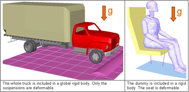
Рисунок 301: Примеры статического равновесия

Объединение жестких тел

Опция /MERGE/RBODY может использоваться для объединения жестких тел вместе или добавления вторичных узлов к существующему жесткому телу. Вторичные сущности, определенные, становятся вторичными по отношению к основному жесткому телу. Вторичные сущности могут быть жесткими телами, отдельными узлами или наборами узлов. Несколько вторичных сущностей могут быть объединены в одно основное жесткое тело путем определения нескольких строк в /MERGE/RBODY.

Некоторые варианты использования включают объединение двух разных сборок, определенных в двух отдельных включаемых файлах, путем определения объединения в основном входном файле. Это также может быть полезно, когда отдельные части, определенные как жесткие, необходимо объединить в одно жесткое тело для моделирования сложного компонента, например, двигателя. Основное твердое тело, определенное в /MERGE/RBODY, может быть определено как вторичное твердое тело в другом

/MERGE/RBODY. Однако следует избегать сложных иерархий, поскольку их может быть трудно отладить. Вторичные сущности могут быть определены только в одном /MERGE/RBODY, а не в любом /RBODY; в противном случае возникают несовместимые кинематические условия.

Перед объединением инерция, масса и центр тяжести каждого вторичного и основного твердого тела рассчитываются на основе их свойств /RBODY. Затем вторичные сущности объединяются с основным твердым телом, и новые свойства твердого тела рассчитываются на основе опции /MERGE/RBODY Iflag.

Жесткая стена (/RWALL)

Жесткая стена — это узловое ограничение, применяемое к набору вторичных узлов, чтобы избежать проникновения узла в стену. Если контакт обнаружен, то ускорение и скорость вторичного узла изменяются.

Нет зазора, чтобы определить, находится ли вторичный узел в контакте. Контакт происходит только тогда, когда вторичный узел соприкасается с жесткой поверхностью стены. Тангенциальная скорость вторичного узла также может изменяться в зависимости от флага Скольжение. Значение по умолчанию (=0) включает чистое скольжение модели во время контакта. Если установлено значение 1, скольжение не допускается, вторичные узлы «связаны» в тангенциальном направлении. Если установлено значение 2, включается трение на основе модели Кулона.

В PRADIOS доступны четыре типа жестких стен:

Бесконечная жесткая стена

• Бесконечная цилиндрическая стена

• Сферическая стена

• Конечная плоская стена

Жесткие стены могут быть фиксированными или подвижными. Фиксированная стена — это чистое кинематическое условие для всех затронутых узлов; тогда как подвижная стена похожа на основной вторичный вариант. Основной узел определяет положение стены на каждом временном шаге и накладывает скорость на затронутые вторичные узлы. Силы затронутого вторичного узла применяются к основному узлу. Силы вторичного узла вычисляются с сохранением импульса. Масса вторичного узла не передается на основной узел, предполагая большую массу жесткой стены по сравнению с массой затронутых вторичных узлов.

Бесконечная жесткая стена

Бесконечная жесткая стена — это плоская поверхность, которая простирается до бесконечности. Она определяется двумя точками, представляющими нормаль жесткой стены (рисунок 302).

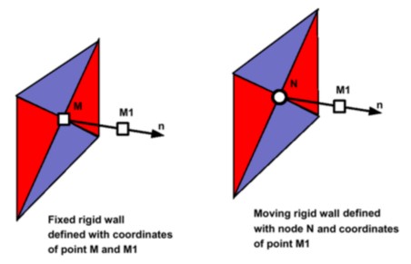
Рисунок 302: Бесконечная жесткая стена

Бесконечная цилиндрическая стена

Бесконечная цилиндрическая стена — это цилиндр, который простирается до бесконечности. Она определяется двумя точками (или одной точкой и одним узлом) и диаметром.

Примечание: контакт возможен только снаружи цилиндрической стенки.

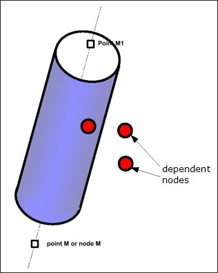
Рисунок 303: Бесконечная цилиндрическая стена

Сферическая стена

Сферическая стена — это сфера, определяемая точкой M (или узлом N) и диаметром.

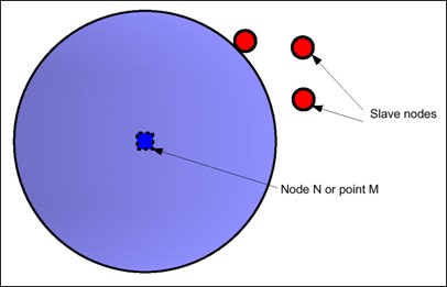
Рисунок 304: Сферическая стена

Конечная плоская стена

Конечная плоская стена — это параллелограмм, определяемый тремя точками M, M1 и M2. В случае движущейся стены M будет считаться основным узлом. .. image:: vertopal_7197fe79ded4471fa6ba70c4c62a5530/media/image49.jpg

width

3.09336in

height

3.33292in

Рисунок 305: Конечная плоская жесткая стена

Комментарии

1. Во время моделирования движущаяся стена следует основному узлу N, но ориентация стены остается постоянной и параллельной исходной нормали. Движущаяся жесткая стена не соблюдает равновесие моментов, применяется только равновесие сил. Внешний момент; поэтому прикладывается из лаборатории к стене.

2.Если вторичные узлы определены только с расстоянием от стенки, то учитываются узлы с положительным или нулевым расстоянием (то есть узлы за бесконечной стеной или в стенке цилиндра не считаются вторичными).

3. Узел, изначально ударившийся о стену, не может отскочить; за исключением случаев, когда скорость отскока достаточно высока, чтобы выйти из стены всего за один цикл.

4. Если к координатам узла добавляется случайный шум, то начальное положение вторичных узлов изменяется, а для движущейся стены изменяется местоположение стены. Поэтому возможно, что некоторые вторичные узлы с нулевым или близким к нулю расстоянием от стены перемещаются внутрь стены. Если вторичные узлы определены с расстоянием, то эти узлы не являются вторичными узлами. Если эти узлы являются явными вторичными узлами, то они останутся внутри стены без возможного отскока.

5. При случайном шуме (/RANDOM) ориентация движущейся стены также изменяется. Местоположение главного узла N перемещается со случайным значением, а нормаль, определенная узлом N и точкой M1, изменяется. Это особенно критично, если точка M1 находится близко к точке N.

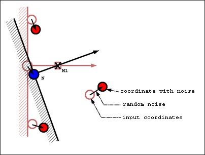
Рисунок 306: Изменение ориентации стены из-за случайного шума

Связанный контакт (/INTER/TYPE2)

Интерфейс TYPE2, также называемый связанным интерфейсом, является узловым ограничением для жесткого соединения набора вторичных узлов с основной поверхностью. Силы и моменты вторичных узлов передаются основным узлам, а затем вторичные узлы позиционируются кинематически в соответствии с движением основных узлов.

Этот интерфейс обеспечивает полное равновесие сил и моментов.

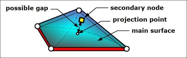
Рисунок 307: Интерфейс TYPE2 - Связанный

Для описания этого соединения доступны четыре формулировки.

• Формулировка точечной сварки по умолчанию

• Оптимизированная формулировка точечной сварки

• Формулировка с отказом

• Формулировка штрафа

Формуляция точечной сварки по умолчанию

\(Spot_{flag} =0\)

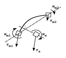
Рисунок 308:

Когда флаг установлен на 0, формулировка spotflag является формулировкой по умолчанию:

• На основе функций формы элемента

• Генерация песочных часов с недоинтегрированными элементами

• Задание функции жесткости соединения вторичной локализации узла

• Рекомендуется для полностью интегрированных оболочек (основных)

• Рекомендуется для соединения вторичных узлов кирпича с основными сегментами кирпича (переход сетки без свободы вращения)

Оптимизированная формулировка точечной сварки

\(Spot_{flag} =1\)

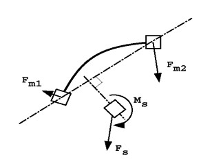
Рисунок 309:

Когда флаг установлен на 1, формулировка spotflag является оптимизированной формулировкой:

• Основана на среднем жестком движении элемента

• Нет проблемы песочных часов

• Постоянная жесткость соединения

• Рекомендуется для недоинтегрированных оболочек (основных)

• Рекомендуется для соединения балок, пружин и вторичных узлов оболочки с основными сегментами кирпича

Формулировка с отказом

\(Spot_{flag}\) =20, 21 and 22

Используя эти опции, можно определить эти два критерия отказа:

Rupt= 0 (независимые параметры разрыва):

Ошибка при достижении Max_N_Dist или Max_T_Dist (по умолчанию)

Rupt= 1 (параметры связанного разрыва):

Ошибка, когда \(\sqrt{\left(\frac{N\_Dist}{Max\_N\_Dist}\right)^{2}+\left(\frac{T\_Dist}{Max\_T\_Dist}\right)^{2}}>1\)

Во время расчета вычисляются нормальное напряжение, касательное напряжение, нормальное смещение и касательное смещение, которые сравниваются с максимальными значениями, определенными в интерфейсе. Как только будут достигнуты максимальные критерии, нормальное напряжение и касательное напряжение будут установлены на 0.

Формулировка штрафа

\(Spot_{flag} = 25\)

Основная цель интерфейса TYPE2 с использованием метода штрафа — привязать вторичный узел к основному сегменту без каких-либо кинематических ограничений. Использование метода штрафа может помочь избежать

“INCOMPATIBLE KINEMATIC CONDITIONS” .

Цилиндрическое соединение (/CYL_JOINT)

Цилиндрическое соединение похоже на твердое тело, за исключением того, что одно конкретное направление определяется первыми двумя вторичными узлами. Все узлы могут свободно перемещаться вдоль этого направления и вращаться вокруг него.

Кинетическое условие применяется ко всем вторичным узлам, включая первые два, определяющие привилегированное направление. Главный узел не используется.

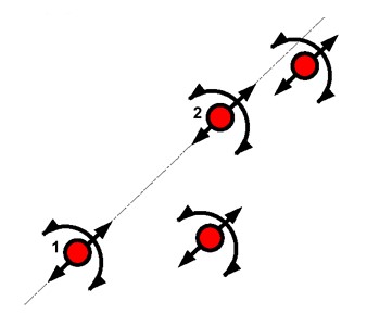
Рисунок 310: Цилиндрическое соединение

Если все вторичные узлы изначально выровнены, они всегда останутся выровненными. Как показано на рисунке 310, свобода вращения — это локальное вращение для каждого узла, а не глобальное вращение вокруг оси 1-2. Поэтому рекомендуется использовать цилиндрическое соединение с выровненными узлами.

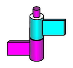
Рисунок 311: Пример дверной петли

Рисунок 311 показывает, как можно смоделировать петлю с помощью цилиндрического соединения. Цилиндрическое соединение состоит из узлов 2, 5, 3 и 4. Обратите внимание, что при моделировании петли узлы должны быть выровнены, чтобы получить реалистичное вращение, затем для соединения узлов 1-2, 2-5, 4-3 и узлов 3-6 используются балки или любые другие конечные элементы. Наконец, можно связать узлы 2-3 с помощью нелинейной упругой пружины, чтобы улучшить соединение.

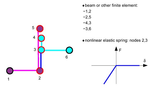
Рисунок 312: Моделирование шарнира

Жесткая связь (/RLINK)

Опция жесткой связи устанавливает одинаковую скорость для всех вторичных узлов для одного или нескольких направлений. Направления определяются для наклонной или глобальной системы координат, скорость вычисляется с сохранением импульса.

Глобальное равновесие моментов не соблюдается. Жесткая связь эквивалентна бесконечной жесткой пружине TYPE8.

Note: A rigid link is a PRADIOS Engine input. A rigid link is alive only during the current restart run. For permanent rigid bodies, the input has to be repeated in each Engine input deck.

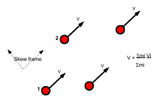
Рисунок 313: Модель жесткой связи

Многоточечные ограничения (/MPC)

Шины зубчатого типа сложнее других кинематических соединений. Они используют метод множителей Лагранжа и совместимы со всеми другими кинематическими условиями множителей Лагранжа и несовместимы со всеми классическими кинематическими условиями.

Приводятся три примера таких соединений:

• Вращающееся зубчатое соединение

• Реечное соединение

• Соединение шестерни дифференциала

Масса и инерция могут быть добавлены ко всем узлам. Соединения MPC накладывают соотношения между скоростями узлов. MPC не может быть применен к поступательным степеням свободы узла без массы или вращательным степеням свободы узла без инерции.

Соединение типа вращательной шестерни

Это сочленение используется для наложения соотношения вращательной скорости между входным и выходным узлом как:

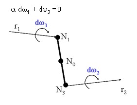
Рисунок 314: Вращательное соединение

Поступательные скорости узлов зубчатого соединения ограничены жестким отношением связи. Для вращательных степеней свободы масштабный коэффициент накладывается между скоростями узлов N₁ и N₂, измеренными в их локальных координатах. Соответствующие уравнения ограничений:

\(d\big{(}\Delta\omega_{1}\cdot r_{1}\big{)}+\big{(}\Delta\omega_{2}\cdot r_{2}\big{)}=0\)

\(\Delta\omega_{1}\cdot s_{1}=0, \Delta\omega_{2}\cdot s_{2}=0\Delta\omega_{1}\cdot t_{1}=0, \Delta\omega_{2}\cdot t_{2}=0\)

Где, \(\Delta\omega_{1}=\omega_{1}-\omega_{0},\) \(\Delta\omega_{2}=\omega_{2}-\omega_{0}\) относительные скорости вращения узлов \(N_{1}\) и \(N_{2}\) по отношению к скорости вращения твердого тела.

Соединение реечной передачи

Это соединение позволяет преобразовать скорость вращения узла в поступательную скорость как: .. image:: vertopal_7197fe79ded4471fa6ba70c4c62a5530/media/image59.jpg

width

3.75994in

height

1.61437in

Рисунок 315: Сочленение типа «рейка и шестерня»

Уравнения ограничений для этих скоростей:

\[\Delta\omega_{1}=\omega_{1}-\omega_{0}, \Delta\omega_{2}=\omega_{2}-\omega_{0}\tag{207}\]

\[a\big{(}\Delta\omega_{0}\cdot s_{1}\big{)}+\big{(}\Delta V_{2}\cdot s_{2}\big{)}=0 \tag{208}\]

\[a\big{(}\Delta\omega_{1}\cdot t_{1}\big{)}+\big{(}\Delta V_{2}\cdot t_{2}\big{)}=0 \tag{209}\]

Дифференциальное соединение зубчатой ​​передачи

Это соединение используется для наложения соотношений скорости вращения между входным узлом и двумя выходными узлами как:

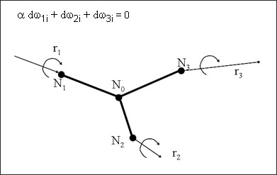
Рисунок 316: Тип дифференциального соединения

Скорости вращения дифференциального соединения ограничиваются соотношениями:

\[d\big{(}\Delta\omega_{1}\cdot r_{1}\big{)}+\big{(}\Delta\omega_{2}\cdot r_{2}\big{)}+\big{(}\Delta\omega_{3}\cdot r_{3}\big{)}=0\tag{210}\]

\[d\big{(}\Delta\omega_{1}\cdot s_{1}\big{)}+\big{(}\Delta\omega_{2}\cdot s_{2}\big{)}+\big{(}\Delta\omega_{3}\cdot s_{3}\big{)}=0\tag{211}\]

\[d\big{(}\Delta\omega_{1}\cdot t_{1}\big{)}+\big{(}\Delta\omega_{2}\cdot t_{2}\big{)}+\big{(}\Delta\omega_{3}\cdot t_{3}\big{)}=0\tag{212}\]

Методы применения кинематических условий

Численные методы, доступные в PRADIOS для применения кинематических условий,

это:

Метод штрафа (жесткие стены)

Смещения узлов ограничиваются применением штрафных сил.

Основное вторичное кинематическое условие (интерфейс TYPE2 и твердое тело)

Все вторичные узлы теряют свою независимость. Степени свободы вторичных узлов

выражаются как функция основного узла или элемента.

Локальное кинематическое состояние (жесткое звено и цилиндрический шарнир)

Уравнения ограничений применяются к узлам для удовлетворения локальных кинематических условий. Главный узел не используется.

Множитель Лагранжа (PRADIOS V44)

Этот метод заключается в нелинейном разрешении уравнений равновесия

при ограничениях. Этот метод является необязательным для некоторых

классических кинематических условий, таких как: интерфейсы, жесткая стенка, жесткое тело

и граничные условия. Это уникальный метод, который доступен для

некоторых новых кинематических условий, таких как: зубчатые соединения и интерфейс

TYPE16 и TYPE17.

Этот метод обычно используется, когда другие методы неприменимы.

Например, когда кинематическое условие должно быть выполнено точно

при контакте узла с поверхностью. С другой стороны, поскольку метод

основан на нелинейном разрешении уравнений методом Ньютона-Рафсона,

его эффективность может быть низкой для общего случая.

Несовместимые кинематические условия

Поскольку узловые ограничения основаны на кинематических условиях, применяемых к узловым степеням свободы, поэтому не допускается применение двух узловых ограничений к одному и тому же набору узлов, если только индуцированные кинематические условия не являются идеально ортогональными (например: граничное условие в направлении X и жесткая связь в направлении Y).

PRADIOS Starter будет выдавать следующее предупреждение каждый раз, когда два узловых ограничения применяются к одному и тому же набору узлов. +———————————————————————–+ | ПРЕДУПРЕЖДЕНИЕ ИДЕНТИФИКАТОР: 147 | | | | *** ВНИМАНИЕ: НЕСОВМЕСТИМЫЕ КИНЕМАТИЧЕСКИЕ УСЛОВИЯ | | | | 2 КИНЕМАТИЧЕСКИХ УСЛОВИЯ НА УЗЛЕ xxxxxx, | | | | В НАПРАВЛЕНИИ ПЕРЕМЕЩЕНИЯ X, ДЛЯ: | | | | - Узловое ограничение 1 (например, ГРАНИЧНОЕ УСЛОВИЕ) | | | | - Узловое ограничение 2 (например, ЖЕСТКАЯ СТЕНА) | +———————————————————————–+

Очень важно учитывать все предупреждения о несовместимых кинематических условиях. Истинно несовместимые кинематические условия (то есть узлы, принадлежащие нескольким твердым телам) могут генерировать энергию и локальную неустойчивость. В таком случае точность результатов будет серьезно снижена.

PRADIOS Starter не проверяет, действительно ли кинематические условия несовместимы. Если они строго ортогональны или если они не применяются одновременно, просто игнорируйте предупреждение. На рисунке 317 показаны два случая: в первом случае узел является вторичным на жесткой стенке и имеет граничное условие в неортогональном направлении. Если жесткая стенка закреплена, то возможных несовместимых условий нет (узел не может удариться о стену). Если стена движется, то невозможно после удара соблюдать оба условия. Поэтому граничное условие не применяется, а силы реакции на стене неверны. Во втором случае узел определяется как вторичный для двух параллельных стенок. Если две жесткие стены зафиксированы, то нет возможных несовместимых условий, поскольку узел не может воздействовать на две стены одновременно. Если одна стена движется, это не приводит к проблемам, пока движущаяся стена не пересекает фиксированную стену.

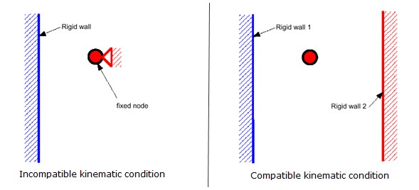
Рисунок 317: Предупреждение PRADIOS о кинематических условиях

В многопроцессорной версии PRADIOS запуск, выполненный дважды, может дать разные результаты, если некоторые кинематические условия несовместимы. Это все еще верно, если используется опция /PARITH/ON. Например, если вторичный узел воздействует на две неортогональные жесткие стенки, как показано на Рисунок 318, результаты, полученные на многопроцессорном компьютере, могут быть произвольными. Если жесткая стенка 1 вычисляется до жесткой стенки 2, скорость V0 заменяется скоростью V12. Если жесткая стенка 2 вычисляется до жесткой стенки 1, скорость V0 становится V21. На многопроцессорных компьютерах порядок, в котором применяются жесткие стенки и другие кинематические условия, произвольный и может быть изменен от одного цикла к другому и от одного запуска к другому.

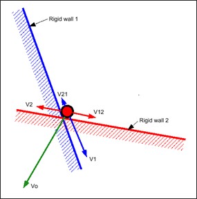
Рисунок 318: Произвольные результаты с несовместимыми кинематическими условиями

Метод множителей Лагранжа позволяет применять несколько узловых ограничений к одному и тому же набору узлов, поскольку он решает глобальную систему уравнений со всеми ограничениями множителей Лагранжа. Однако не допускается смешивать оба метода для одного и того же набора узлов. Тем не менее, оба метода можно успешно использовать в модели, если они применяются к разным узлам.

В PRADIOS доступно несколько интерфейсов, в этом разделе рассматриваются только контактные интерфейсы. Каждый интерфейс отличается номером типа.

Интерфейс TYPE2 — это кинематическое условие, используемое для соединения двух сеток Лагранжа, и в этом разделе не описывается подробно (см. Кинематические ограничения). Краткий обзор контактных интерфейсов показан в Таблице 21.

Каждый из этих интерфейсов был разработан для определенной области применения, но эта область — не единственный критерий выбора. Некоторые ограничения различных алгоритмов, используемых в каждом интерфейсе, также могут определить ваш выбор.

Ограничения алгоритма в основном касаются поиска затронутого сегмента. Этот поиск можно выполнить напрямую (интерфейс TYPE7, TYPE10 и TYPE11) или через поиск ближайшего узла (другие типы интерфейсов). Поиск ближайшего узла выполняется с помощью дешевого, но ограниченного алгоритма (интерфейс TYPE3, TYPE5 и TYPE6).

Интерфейсы TYPE3, TYPE5 и TYPE6 также имеют некоторые ограничения, касающиеся выбора между сегментами, подключенными к ближайшему узлу. Нормальная ориентация является одним из ограничений для этих интерфейсов.

Интерфейс TYPE23 определяет контактный интерфейс для тканей подушек безопасности. Это мягкий штрафной контакт, который может иметь дело с проникновением и пересечением, часто возникающими в сложенной сетке подушки безопасности.

Интерфейс TYPE24 использует постоянную штрафную жесткость, и поэтому временной шаг не влияет.

Тепловое трение можно вычислить с помощью интерфейсов TYPE7 и TYPE21.

Таблица 21: Интерфейсы в PRADIOS

Тип	Описание	Приложение	**Контакт Уход **
1 / 9	ALE/LAG с скользящий	Fluid-structure взаимодействие	Основное- Вторичное
2	Связанный интерфейс	Изменение сетки density (твердый)	Основное- Вторичное или LM

| | (твердый) | |

Воздействие | использовать | Штраф |

| между двумя | рекомендуется | |

| частями | TYPE7 | |

Воздействие | Пользовательский| Штраф |

| между двумя | Контакты | |

| твердые тела | | |

7	Общий цель Контакт Воздей- ствие между двумя частями	твердый Контакт Воздействие на все скорости	Штраф или LM
8	Вытяжка контакт	Штамповка приложения	Штраф
10	Как TYPE7, но привязан Контакт	Специальный цель интерфейс	Штраф
11	Удар между двух линий	стержни или пружины
12	Жидкость/жид- кость Контакт	Жидкость/жид- кость Контакт	Штраф
16 & 17	Контакт между узлами в квадратный твердые тела формы и твердые оболочки или между квад- ратные формы	Сетки с 8-узловой или 16узлов толстостенный или 20 кирпичей	LM
18	CEL Лагранж / Эйлер интерфейс	Жидкостная структура взаимодействия	Штраф
19	Сочетание интерфейс TYPE7 и TYPE11	Твердый Контакт влияние вообще скорости и Для балки, стержни или пружины	Штраф
21	Специфический интерфейс между недеформируемый основная поверхность и вторичный поверхность	Для штамповки	Основной-Вторичный
23	мягкий Штраф Контакт	Для подушки безопасности	мягкий Штраф
24	общий контакт интерфейс, необязательный одинарная по- верхность или поверхность поверхность или узлы для поверхность контактов	этот контакт интерфейс может заменить интерфейс TYPE3, 5, 7	Штраф жесткость константу и; следовательно, шаг по времени не затронуто

Обработка контакта

Существует два подхода, которые работают с контактом:

• Метод штрафа чаще всего используется в явных кодах и может быть найден в большинстве интерфейсов PRADIOS

• Метод множителей Лагранжа (/LAGMUL и /INTER/LAGMUL) используется в специальных исследованиях случаев

Метод штрафа

Интерфейсы, использующие метод штрафа, основаны на основной/вторичной обработке. Контакт может происходить только между набором вторичных узлов и набором основных сегментов. Основные сегменты определяются в зависимости от типа элемента, на котором они лежат. Если это 3-узловая или 4-узловая оболочка, сегмент является поверхностью элемента. Если это сплошной элемент, сегмент определяется как грань. Наконец, если это 2D-сплошной элемент (квадрат), сегмент является стороной.

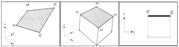
Рисунок 319: Определение сегмента

Расстояние зазора определяется для определения того, находится ли узел в контакте с сегментом.

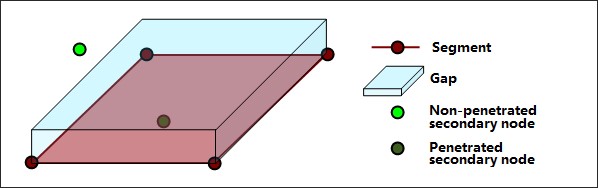
Рисунок 320: Зазор и проникновение

Как только узел проникает в зазор, упругая пружина добавляется между вторичным узлом и основным сегментом. Поэтому сила сопротивления будет стремиться отклонить вторичный узел.

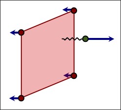
Рисунок 321: Сила реакции в интерфейсе

На временной шаг может влиять жесткость интерфейса. Во время проникновения, поскольку пружина соединена с вторичным узлом, жесткость пружины должна быть добавлена ​​к общей жесткости, действующей на узел (жесткость от всех элементов, соединенных с этим узлом). Узловой временной шаг должен быть уменьшен для учета жесткости пружины.

\[dt=\sqrt{\frac{2M_{node}}{K_{node}+K_{spring}}}\tag{213}\]

Контакт заканчивается, когда проникший узел полностью выталкивается из зазора. Таким образом, упругая пружина и сила реакции удаляются.

Стоит отметить, что контактные интерфейсы с методом штрафа полностью совместимы со всеми кинематическими условиями (например, жесткое тело, приложенная скорость и т. д.).

Метод множителей Лагранжа(/LAGMUL and /INTER/LAGMUL)

В отличие от метода штрафа, метод множителей Лагранжа является чисто математическим и не требует физических элементов (пружин) для моделирования контакта. Нелинейная система уравнений решается для учета контактных условий. Поэтому нет коллапса временного шага из-за высокой жесткости интерфейса, но требуется больше времени ЦП для выполнения одного цикла, так как новые уравнения должны быть решены нелинейным решателем. Метод имеет преимущество в остановке вторичных узлов на контактной поверхности (условие контакта точно выполняется); однако трение не может быть вычислено.

Симметричный интерфейс (/INTER/TYPE3)

Этот интерфейс используется для моделирования симметричных ударов между двумя поверхностями.

Обе поверхности определяются с помощью использования ориентированных сегментов; поэтому контакты могут происходить только с одной стороны. Каждый узел на обеих поверхностях рассматривается как вторичный узел, а каждая поверхность рассматривается как основной сегмент.

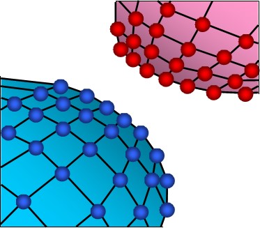
Рисунок 322: Интерфейс TYPE3

В отличие от интерфейса TYPE5, интерфейс TYPE3 имеет две основные поверхности; поэтому алгоритм контакта выполняется дважды. Первый проход решает проникновение узлов с первой поверхности относительно второй поверхности. Второй проход решает проникновение узлов со второй поверхности относительно первой поверхности. Это приводит к более высокой точности по сравнению с интерфейсом TYPE5, но требуется больше времени ЦП.

При обнаружении контакта добавляется упругая пружина, и жесткость пружины рассчитывается с использованием жесткости обеих поверхностей. На основе материальных и геометрических свойств жесткость приписывается каждой поверхности, затем вычисляется общая жесткость интерфейса:

\[K=s\frac{K_{1}K_{2}}{K_{1}+K_{2}}\tag{214}\]

Значение по умолчанию для масштабного коэффициента(ов) жесткости равно 0,2, по соображениям устойчивости это значение не следует изменять. Однако, если соотношение \(K_{1}\) к \(K_{2}\) больше 100 (или меньше 0,01), рекомендуется увеличить масштабный коэффициент жесткости, чтобы избежать слишком многочисленных проникновений. Жесткость пружины постоянна, что позволяет вторичным узлам проходить через среднюю плоскость основного сегмента.

Этот интерфейс не позволяет выполнять моделирование автоконтакта, поскольку узел не может принадлежать обеим поверхностям.

Примечание: Этот интерфейс в основном используется для пластин оболочки изначально находящихся в контакте. Если две пластины моделируются с зазором между двумя сетками, лучше использовать интерфейс TYPE7; если только, если две пластины моделируются без зазора, интерфейс TYPE3 является хорошим выбором.

Несимметричный интерфейс (/INTER/TYPE5)

Этот интерфейс используется для моделирования ударов между основной поверхностью и списком вторичных узлов.

Интерфейс ориентирован; поэтому контакт может происходить только с одной стороны основных сегментов. Таким образом, нормаль основных сегментов должна быть ориентирована к вторичным узлам.

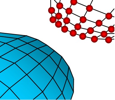
Рисунок 323: Интерфейс TYPE5

Основная сетка поверхности должна быть регулярной с хорошим соотношением сторон. Не допускается размещение вторичного узла на основной поверхности. Он работает только с основными сегментами, соединенными с твердыми или оболочечными элементами. Одним из вариантов использования этого интерфейса является замена жесткой стенки. Замена жесткой стенки на интерфейс TYPE5 позволит вам моделировать удары жесткого тела.

С интерфейсом TYPE5 зазор используется для определения контакта между узлом и поверхностью. Этот зазор определяется пользователем и расположен на стороне, нормальной к поверхности. Рекомендуется использовать небольшой или нулевой зазор.

При обнаружении контакта добавляется упругая пружина, и жесткость пружины рассчитывается с использованием только материальных и геометрических свойств основного сегмента. В целях обеспечения устойчивости к жесткости основной стороны применяется масштабный коэффициент жесткости 0,2. Настоятельно рекомендуется не изменять этот коэффициент, если только основная сторона не очень мягкая по сравнению с второстепенной стороной. В этом случае рекомендуется использовать отношение большего модуля упругости к меньшему в качестве масштабного коэффициента жесткости.

Как упоминалось ранее, жесткость зависит от геометрических и материальных свойств, а также от типа элемента. На рисунке 324 описывается способ расчета жесткости в соответствии с типом элемента, к которому прикреплен сегмент. В случае, если сегмент является общим для кирпича и оболочки (например: 3D-деталь, покрытая оболочкой), используется жесткость, связанная с элементом оболочки.

Рисунок 324: Жесткость в интерфейсе TYPE5

Главный недостаток интерфейса TYPE5 заключается в том, что контакт не может происходить с обеих сторон основного сегмента. Для проблемы с большими поворотами (обычно это происходит при анализе столкновений) контакт, скорее всего, произойдет с неправильной стороны поверхности; поэтому проникновение не будет обнаружено. Следовательно, для сложной проблемы контакта необходимо хорошее понимание удара до моделирования, чтобы правильно определить нормальные поверхности.

Другой важный недостаток заключается в том, что узел не может быть вторичным узлом и частью основного сегмента. Поэтому автоконтакт не может быть смоделирован с использованием интерфейса TYPE5.

Распространенные проблемы в интерфейсах TYPE3 и TYPE5

Интерфейсы TYPE3 и TYPE5 имеют некоторые общие проблемы.

• Скачки энергии

• Плохая обработка контактов

• Ограниченный алгоритм поиска

Скачки энергии

Зазор, используемый в интерфейсе TYPE5 (и TYPE3), является односторонним и не учитывает края. Это может привести к скачкам энергии в случаях большого зазора (рисунок 325).

Рисунок 325: Скачок энергии

Плохая обработка контакта

Более того, поскольку жесткость интерфейса постоянна, допускается проникновение узла. Эта точка может привести к огромной ошибке, особенно если скольжение происходит во время проникновения. Рисунок 326 иллюстрирует, как вторичные узлы могут проходить через середину поверхности оболочки из-за плохой обработки контакта.

Рисунок 326: Обработка плохого контакта

Ограниченный алгоритм поиска

С интерфейсом TYPE5 (и TYPE3) обнаружение ближайшего основного узла ограничено сегментами, топологически близкими к предыдущему (топологически ограниченный алгоритм поиска). Первый поиск выполняется PRADIOS Starter для определения ближайшего начального основного узла, затем Engine определяет ближайший основной узел, принимая во внимание только сегменты, топологически близкие к предыдущему. Этот метод довольно медленный по времени ЦП, и он не очень хорошо работает, особенно если задействованы высокие кривизны (Рисунок 327).

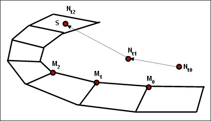
Рисунок 327: Плохое обнаружение ближайшего основного сегмента

Интерфейс TYPE6 (/INTER/TYPE6)

Интерфейс TYPE6 используется для моделирования контакта между двумя твердыми телами.

Этот интерфейс похож на интерфейс TYPE3, за исключением жесткости. Взаимосвязь между контактной силой и проникновением обеспечивается определяемой пользователем функцией. Этот интерфейс используется, в частности, в моделировании пассажиров транспортных средств, например: коленных буферов. Основное ограничение этого интерфейса заключается в том, что поверхность 1 должна быть частью одного твердого тела, а также для поверхности 2. Более того, обе поверхности должны быть ориентированы так, чтобы нормали были обращены друг к другу.

Используемая жесткость соответствует кривой Сила против Проникновения, введенной вами. Мгновенная жесткость интерфейса представляет собой наклон входной кривой при заданном проникновении; поэтому временной шаг может быть влиян, поскольку жесткость интерфейса используется для вычисления стабильного временного шага:

\[\Delta t=0.1\sqrt{\frac{M}{K}}\tag{215}\]

Где,

\(M\) The min (Масса первого твердого тела и Масса второго твердого тела)

\(K\) Наклон кривой силы против проникновения

Рисунок 328: Интерфейс TYPE6 — Нормальная ориентация

Интерфейс общего назначения (/INTER/TYPE7)

Интерфейс TYPE7 — это интерфейс общего назначения, который может имитировать все типы удара между набором узлов и основной поверхностью. В отличие от интерфейсов TYPE3 и TYPE5, интерфейс TYPE7 не ориентирован, и вторичные узлы могут принадлежать основной поверхности. Поэтому этот интерфейс может имитировать самоудар, особенно выпучивание при столкновении на высокой скорости.

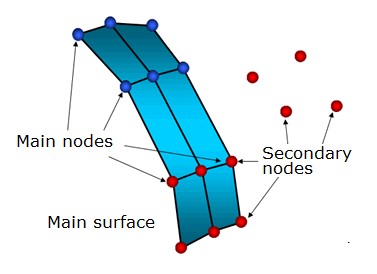
Рисунок 329: Интерфейс TYPE7

Интерфейс TYPE7 решает все проблемы и ограничения, возникающие с интерфейсом TYPE3 и TYPE5. Поиск ближайшего сегмента выполняется с помощью алгоритма прямого поиска; поэтому ограничений поиска нет, и находятся все возможные контакты. Скачки энергии, вызванные узлом, ударяющимся о края оболочки, устраняются использованием цилиндрического зазора вокруг краев.

Наконец, главное преимущество интерфейса TYPE7 заключается в том, что жесткость не является постоянной и увеличивается с проникновением, предотвращая прохождение узла через середину поверхности оболочки. Это решает многие проблемы с плохим контактом (распространенные при использовании интерфейса TYPE3 или TYPE5).

Зазор, используемый в интерфейсе TYPE7, довольно сильно отличается от зазоров предыдущих интерфейсов. Зазор используется по обе стороны от средней поверхности оболочки, а вокруг краев добавляется цилиндрический зазор (рисунок 330). Зазор используется по обе стороны от средней поверхности оболочки, а вокруг краев добавляется цилиндрический зазор.

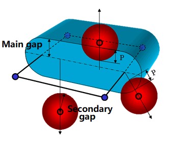
Рисунок 330: Зазор в интерфейсе TYPE7

Цилиндрический зазор позволяет избавиться от скачков энергии, узлы, воздействующие с краев, следуют по тому же пути при проникновении и выходе. Более того, такой зазор сохраняет силу реакции плавной при скольжении между сегментами.

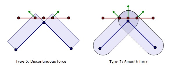
Рисунок 331: Скольжение между сегментами

В отличие от интерфейса TYPE3 и TYPE5, переменный зазор в пространстве доступен. В зависимости от опции \(I_{gap}\), переменный зазор вычисляется для каждого удара как сумма основного зазора элемента (g_m) и зазора вторичного узла (g_s).

Если \(I_{gap}\) =1, переменный зазор вычисляется как: .. math:: maxBigl{[}Gap_{min},Bigl{(}g_{s}+g_{m}Bigr{)}Bigr{]}tag{216}

Если \(I_{gap}\) =2, переменный зазор вычисляется как:

\[\max\Bigl{\{}Gap_{min},\min\Bigl{[}Fscale_{gap}\cdot\Bigl{(}g_{s}+g_{m}\Bigr{)} Gap_{max}\Bigr{]}\Bigr{\}}\tag{217}\]

Если \(I_{gap}\) =3, переменный зазор вычисляется как:

\[\max\Bigl{\{}Gap_{min},\min\Bigl{[}Fscale_{gap}\cdot\Bigl{(}g_{s}+g_{m},\Bigr{)} ,\text{%mesh_size}\cdot\Bigl{(}g_{s\_s}+g_{m\_l}\Bigr{)}, Gap_{max}\Bigr{]}\Bigr{\}}\tag{218}\]

Таблица 22: Расчет переменного зазора

Элемент	главный Элемент Зазор gm	**Вторичный узел Зазор** gs
ОБОЛОЧКА	\(g_{m}=\frac{t} {2}\) t: толщина главног осегмента	\(g_{s}=\frac{t} {2}\) t: наибольшая толщина оболочка эелемента подключен к sвторичному узлу
брусок	gm = 0	gm = 0
ФЕРМА и БАЛКА	Неприменимо	\(g_{s}=\frac{1} {2}\sqrt{S}\) S: поперечное сечение

Если также используется минимальный зазор для активации удара (\(Gap_{min}\)), то вычисленный переменный зазор не может быть меньше минимального значения. Также можно применить масштабный коэффициент к зазору и определить максимальное значение зазора.

Начальные проникновения

В модели FE начальные проникновения очень распространены, неизбежны и являются результатом дискретизации во время процесса построения сетки (рисунок 332).

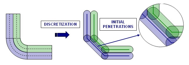
Рисунок 332: Начальные проникновения из-за дискретизации

Inacti

Специальная обработка начальных проникновений может быть выполнена с помощью флага Inacti. Можно удалить проникшие узлы из интерфейса или удалить основные сегменты, относящиеся к проникшим узлам. Оба способа обработки позволяют очень легко избавиться от начальных проникновений, но они могут привести к плохим результатам, если количество проникших узлов велико.

Установка Inacti на 3 позволяет PRADIOS Starter автоматически изменять координаты проникших узлов, чтобы избежать начальных проникновений. При этом следует соблюдать особую осторожность, поскольку эта операция может привести к изначально ограниченным пружинам.

Также можно получить переменный зазор во времени, установив Inacti на 5. Иллюстрация на рисунке 333 объясняет, как эффективный зазор обновляется с учетом предыдущих проникновений.

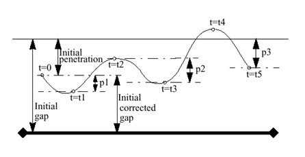
Рисунок 333: Переменный зазор во времени

В момент t=0, если узел изначально проникает, его зазор автоматически исправляется. Затем этот «начальный исправленный зазор» будет увеличиваться каждый раз, когда узел удаляется от основного сегмента. Эта опция в основном используется для развертывания подушки безопасности, она обеспечивает приличный временной шаг в начале развертывания, тогда как все узлы сильно проникают.

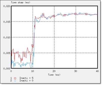
Рисунок 334: Временной шаг с использованием Inacti=5

Чтобы избежать высокочастотных эффектов, рекомендуется Inacti = 6 вместо Inacti =5.

Fpenmax

Fpenmax (максимальная доля начального проникновения) используется для работы с большим начальным проникновением. Жесткость узла будет отключена, если \(Penetration\geq F penmax\cdot Gap,\) , каким бы ни было значение Inacti.

Igap3 + %mesh_size

При \(I_{gap}\) = 3 и %mesh_size можно учесть размер сетки, чтобы избежать начальных проникновений. В этом случае переменная gap вычисляется как:

\[\max\Bigl{\{}Gap_{min},\min\Bigl{[}Fscale_{gap}\cdot\Bigl{(}g_{s}+g_{m},\Bigr{)} ,\text{%mesh_size}\cdot\Bigl{(}g_{s\_l}+g_{m\_l}\Bigr{)}, Gap_{max}\Bigr{]}\Bigr{\}}\tag{219}\]

Где,

\(g_{m\_l}\) Длина меньшего края элемента

\(g_{s\_l}\) Длина меньшего края элементов, соединенных со вторичным узлом

Irem_gap

Опция Irem_gap используется для деактивации вторичных узлов, которые закрывают (Криволинейный \(Расстояние <\sqrt{2}\cdot Зазор\)) элементы. Эта опция полезна для самоударного контакта, когда размер сетки очень мал. .. image:: vertopal_7197fe79ded4471fa6ba70c4c62a5530/media/image79.jpg

width

3.28363in

height

3.34196in

Рисунок 335: -1: Определение Irem_gap

настоятельно рекомендуется |

удалять начальные проникновения во время создания |

|

модели FE, используя инструменты предварительной |

обработки, такие как HyperMesh и |

депенетраторы HyperCrash. |

Жесткость интерфейса

Как и другие типы интерфейсов, при использовании метода штрафа интерфейс имеет пружинную жесткость, поскольку вторичный узел проникает в зазор; однако сила реакции вычисляется с гораздо лучшим приближением. Изменение силы в зависимости от проникновения узла нелинейно из-за возрастающей жесткости.

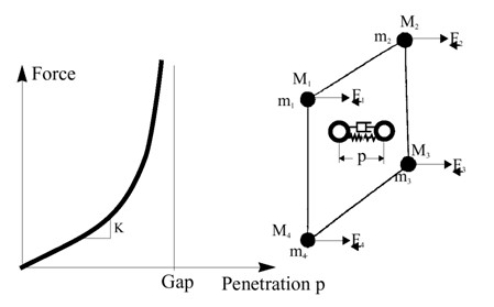
Рисунок 336: Изменение силы интерфейса в интерфейсе TYPE7

Жесткость интерфейса (K) не является постоянной, она увеличивается с проникновением. Более того, существует вязкое демпфирование, действующее на скорость проникновения. Контактная сила затем вычисляется как:

\[\begin{split}F_{n}=K_{S}P+C\frac{dP}{dt}\left\{\begin{array} K_{S}=K_{0}\frac{Gap}{Gap-P} \\ C=VIS_{S}\sqrt{2K_{S}M}\end{array}\right.\end{split}\]

Мгновенная жесткость затем вычисляется как:

\[K_{t}=\frac{\partial F}{\partial P}=K_{0}\frac{Gap^{2}}{\left(Gap-P\right)^{2}}\tag{221}\]

Узловой временной шаг может быть серьезно затронут, если проникновение велико. Жесткость, используемая для вычисления узлового временного шага, учитывает жесткость интерфейса.

Есть два способа уменьшить жесткость интерфейса:

• Увеличение зазора

• Увеличение начальной жесткости (с помощью флага Stfac)

Оба метода позволяют поглощать больше энергии при контакте и сглаживать удар. Увеличение зазора позволит узлам замедляться на большем расстоянии, поэтому проникновение уменьшается.

Комментарии

1. Даже если для моделирования выбран элементарный временной шаг, узловой временной шаг автоматически вычисляется, если есть интерфейс TYPE7. Для моделирования применяется наименьший временной шаг

2. В отличие от интерфейса TYPE5, Stfac меньше 1,0 создает большое проникновение при первом касании и приводит к высокой жесткости интерфейса и силе реакции. Чтобы избежать большого проникновения, рекомендуется Stfac больше или равно 1,0. .. image:: vertopal_7197fe79ded4471fa6ba70c4c62a5530/media/image81.jpg

width

3.57247in

height

2.97879in

Рисунок 337: Кривые зависимости силы от проникновения

Хотя увеличение начальной жесткости приводит к меньшему временному шагу в начале проникновения, это увеличит временной шаг, если проникновение большое.

Трение

В PRADIOS доступно несколько формул трения. Самая простая, которая также является наиболее используемой, — это закон трения Кулона. Эта формулировка обеспечивает точные результаты при анализе столкновений и требует всего одного параметра (коэффициент трения Кулона, \(\mu\)).

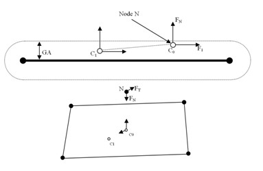
Рисунок 338: Нормальные и касательные силы, приложенные к узлу .. image:: vertopal_7197fe79ded4471fa6ba70c4c62a5530/media/image84.jpg

width

3.85368in

height

2.1664in

Рисунок 339: Расчет силы адгезии

Значение по умолчанию для (:raw-latex:`\mu`) равно 0 (нет трения между поверхностями). Для расчета силы трения формула штрафа за трение по умолчанию является вязкой, основанной на тангенциальной скорости. Во время скользящего проникновения узел переходит из положения (C_{0}) (точка контакта в время (t)) в (C_{1}) (положение контакта в время (t+:raw-latex:`Delta `t)). Поскольку контакт вязкий, для расчета силы адгезии вводится коэффициент вязкости (C):

\[F_{adh}=C\cdot V_{t} \tag{222}\]

Где,

\(C=VIS_{F}\cdot\sqrt{2KM}\)

K

Мгновенная жесткость интерфейса

VIS

_F Критический коэффициент демпфирования трения интерфейса

M

Основная масса узла

После вычисления силы адгезии (F_h), если она меньше, чем \(mu F_{n,}\), сила трения не изменяется, равняясь F_h, и произойдет прилипание. Если сила адгезии больше, чем \(mu F_{n,}\), то сила трения уменьшается и равна \(mu F_{n.}\)

\[F_{t}=\min\bigl{(}\mu F_{n} F_{adh}\bigr{)}\tag{223}\]

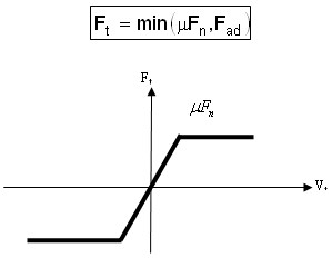
Рисунок 340: Расчет силы трения

Если скольжение происходит на очень низкой скорости (например: квазистатическое моделирование), вязкая формула не будет работать, поскольку сила трения вычисляется по тангенциальной скорости. Чтобы преодолеть это ограничение, доступна новая формула штрафа за трение, основанная на тангенциальном смещении (формула приращения жесткости). Этот метод вводит искусственную жесткость, K, для расчета изменения силы трения:

\[\Delta F_{t}=K\cdot V_{t}\cdot\delta_{t}\tag{224}\]

Где,

\(\delta_{t}\) Смещение по касательной

Поэтому, в отличие от предыдущей формулировки, формулировка жесткости способна вычислить правильную силу трения даже при низкой скорости. Рисунок 341 иллюстрирует этот момент. Если наложенное смещение применяется к детали (трехмерному кубу) при низкой скорости (0,01 м/с), вязкая формуляция не будет работать; тогда как формулировка жесткости, основанная на смещении по касательной, будет.

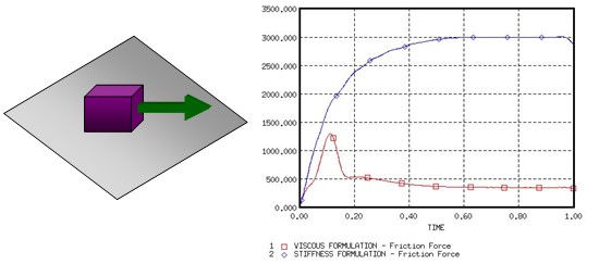
Рисунок 341: Формулировка вязкости против формулы жесткости

Доступны и другие формулы трения, их принцип похож на закон трения Кулона. PRADIOS сначала вычисляет силу адгезии, которая затем сравнивается с \(\mu F_{n}\). Их различия заключаются в коэффициенте трения (\(\mu\)), который больше не является постоянным, а зависит от давления нормальной силы на основной сегмент и от тангенциальной скорости вторичного узла. В зависимости от флага \(I_{\text{{{fric}}}}\) доступны три новые формулы трения:

Обобщенный закон вязкого трения

\[\mu=Fric+C_{1}p+C_{2}\cdot V+C_{3}p\cdot V+C_{4}\cdot p^{2}+C_{5}\cdot V^{2}\tag{225}\]

Модифицированный закон трения Дармстада

\[\mu=Fric+C_{1}\cdot\dot{e}(C_{2}v)\cdot p^{2}+C_{3}\cdot\dot{e}^(C_{4}v)\cdot p+C_{5}\cdot\dot{e}^(C_{6}v)\tag{226}\]

Закон трения Ренара

\[\mu=C_{1}+\left(C_{3}-C_{1}\right)\cdot\frac{V}{C_{5}}\cdot\left(2-\frac{V}{C_{5}}\right)\tag{227}\]

Если

\[V\in\left[C_{5}\cdot C_{6}\right] \tag{228}\]

\[\mu=C_{3}-\left(\left(C_{3}-C_{4}\right)\cdot\left(\frac{V-C_{5}}{C_{6}-C_{5}}\right)^{2}\cdot\left(3-2\cdot\frac{V-C_{5}}{C_{6}-C_{5}}\right)\right)\tag{229}\]

Если

\[V\in\left[C_{5}\cdot C_{6}\right] \tag{230}\]

\[\mu=C_{2}-\frac{1}{\frac{1}{C_{2}-C_{4}}+\left(V-C_{6}\right)^{2}}\tag{231}\]

Если

\[V\geq C_{6} \tag{232}\]

\[P=C_{1}\cdot\mu+C_{4}\cdot\rho\cdot C_{v}\cdot T=C_{1}\cdot\mu+\alpha_{v}\cdot T\tag{233}\]

Примечание: Фильтрация трения доступна для всех типов трения. формулировки и позволяет вам сгладить силу трения. Подробнее см. в разделе PRADIOS Starter Input.

Рисунок 342: Графическое представление модели трения Ренара

Теплообмен

В интерфейсе TYPE7 есть три теплообмена: теплопередача, излучение и тепловое трение разрешены \(I_{the}\) =1.

Для теплопередачи между вторичным и основным с Iform_the можно определить два различных теплообмена. Один из них задает постоянную температуру в интерфейсе, где теплообмен происходит только между этим интерфейсом и вторичной стороной оболочки. Другой — теплообмен между всеми частями в контакте.

Если Frad≠ 0, то излучение вычисляется внутри расстояния Drad (макс. расстояние для вычисления излучения). Рекомендуется не устанавливать слишком большое значение для Drad , иначе производительность PRADIOS Engine может снизиться.

Использование Fheat_s и Fheat_m фрикционной энергии скольжения будет преобразовано в тепло. Поскольку тепло трения делится между вторичной и основной стороной, обычно Fheat_s + Fheat_m < 1,0. Тепло трения Q_Fric определяется:

Если I_Form =2 (формуляция жесткости):

Вторичная сторона: .. math:: Q_{Fric}=Fheat_{s}cdotfrac{left(F_{textit{adh}}-F_{t}right)}{K}cdot F_{t} tag{234}

Основная сторона:

(Ithe_form=1)

Здесь K — это Жесткость контакта \(F_{adh}\)

Если I_Form =1 (формуляция штрафа):

Вторичная сторона:

\[Q_{Fric}=F heat_{s}\cdot C\cdot V_{t}2\cdot dt \tag{236}\]

Основная сторона:

Управление шагом времени интерфейса

В предыдущем разделе объясняется, что шаг времени может быть серьезно уменьшен во время контакта, поскольку жесткость добавляется ко всем проникающим узлам. Более того, чтобы предотвратить прохождение любого узла через основной сегмент в течение одного цикла, также вычисляется кинематический шаг времени. Если скорость удара узла достаточно высока, чтобы пройти через сегмент за один цикл, PRADIOS уменьшает шаг времени, чтобы применить штрафную силу, когда узел находится на расстоянии зазора. Если p — это расстояние проникновения, то dp/dt — это скорость проникновения, а кинематический временной шаг — это необходимое время для того, чтобы узел прошел половину расстояния между узлом и сегментом. Узловой временной шаг также вычисляется для обеспечения численной стабильности. Наименьший временной шаг затем используется для моделирования.

Узловой шаг времени во время контакта:

Кинематический шаг времени: .. math:: dt_{kin}=frac{1}{2}biggl{[}frac{Gap-p}{dp/dt}biggr{]}tag{239}

Если по какой-то причине узел сильно проник, либо шаг по времени узла, либо шаг по времени кинематики может быть очень низким. Тогда можно освободить этот узел от интерфейса, используя опцию /DT/ INTER/DEL в файле Engine. Все узлы, достигающие dt_min, будут удалены из интерфейса.

Увеличение массы

Использование масштабирования массы (/DT/NODA/CST) может привести к нестабильности массы. По мере проникновения узла его глобальная жесткость увеличивается (добавляется мгновенная жесткость интерфейса, K_t); поэтому его узловой шаг по времени уменьшается. Чтобы соответствовать минимальному шагу по времени, PRADIOS добавляет необходимую массу к узлу. К сожалению, эта добавленная масса увеличивает кинетическую энергию, и проникновение становится больше.

Рисунок 343: Влияние масштабирования массы на интерфейс TYPE7

Если интерфейс не способен остановить проникновение, добавленная масса (из-за масштабирования массы) будет продолжать становиться все больше и больше. Поэтому, вычисление, скорее всего, остановится, поскольку изменение массы может стать огромным очень быстро (несколько циклов). Если это так, интерфейс следует модифицировать:

• Зазор следует увеличить

• Начальную жесткость можно увеличить

• Сетку следует модифицировать, чтобы она была более тонкой и однородной в зоне контакта

Мягкая часть против твердой части

Значение жесткости по умолчанию, вычисленное PRADIOS, часто подходит для избежания очень высокого проникновения, приводящего к падению шага по времени. Когда происходит контакт между похожими материалами, нет проблем с использованием жесткости по умолчанию; за исключением случаев, когда материалы различаются. Например, когда мягкая сталь сталкивается с мягкой пеной, жесткость по умолчанию может быть слишком низкой, чтобы избежать большого проникновения. Когда такие контакты желательны, рекомендуется сначала вычислить отношение жесткости вторичного материала к жесткости основного материала. Если это отношение больше 100, следует использовать масштабный коэффициент (Stfac), равный этому отношению, для увеличения жесткости интерфейса.

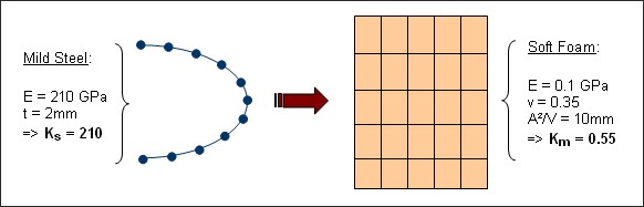
Рисунок 344: Удар между сталью и пеной

На рисунке 344 показан контакт между мягкой сталью и мягкой пеной. Коэффициент жесткости больше 380, в таком случае, когда основная сторона является мягкой стороной, флаг Stfac может быть установлен на 380, чтобы избежать очень высоких проникновений.

Блокировка удара кромка к кромке

Интерфейс TYPE7 не справляется с ударом кромка к кромке. Ограничение этого интерфейса во время контакта кромка к кромке показано на Рисунок 345.

Рисунок 345: Контакт края с краем

Когда сетка достаточно мелкая, за проникновением края с краем часто следует контакт узла с оболочкой. Основная проблема при ударе края с краем — это ситуации блокировки. Если после проникновения края происходит изменение нагрузки, блокировка неизбежна, поскольку обнаруживается контакт узла с поверхностью (Рисунок 346). Обычно это приводит к высокому проникновению; поэтому анализ останавливается по мере уменьшения временного шага. Если происходит блокировка, необходимо использовать интерфейс TYPE11 в этой области для решения проблемы.

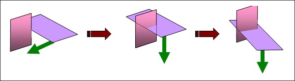
Рисунок 346: Блокировка после проникновения через край

Создание тангенциальной силы

Тангенциальная сила может быть создана, когда проникший узел скользит без трения. Такое поведение обусловлено зазорами, перекрывающимися вокруг краев. Рисунок 347 иллюстрирует, что из-за цилиндрического зазора вокруг краев сила больше не является нормальной к средней поверхности оболочки. .. image:: vertopal_7197fe79ded4471fa6ba70c4c62a5530/media/image92.jpg

width

5.68679in

height

1.78103in

Рисунок 347: Генерация тангенциальной силы

Комментарии

1. Всегда рекомендуется выполнять постобработку контактных сил. Если они слишком велики, принимая во внимание физическое понимание, модель должна быть проверена.

2. Для постобработки сил для симметричного контакта интерфейс можно разделить на четыре интерфейса. Например, для двух частей A и B можно создать: - Интерфейс 1 с A вторичным и B основным

• +Интерфейс 2 с A основным и B вторичным

• +Интерфейс 3 с A основным и вторичным

• +Интерфейс 4 с B основным и вторичным

Предупреждение о зазоре автоматического контакта

Это предупреждение следует принимать во внимание только для самоударного интерфейса.

При моделировании автоконтакта настоятельно рекомендуется использовать минимальный зазор не менее половины наименьшего края сегмента. Сообщение означает, что по крайней мере один элемент на основной стороне имеет длину стороны меньше, чем в два раза больше GAP, и существует риск чрезмерной жесткости.

ИДЕНТИФИКАТОР ПРЕДУПРЕЖДЕНИЯ: 94 ** ПРЕДУПРЕЖДЕНИЕ В ИНТЕРФЕЙСЕ GAP ВХОДНОЙ GAP 1.7 ОДНАКО РЕКОМЕНДУЕТСЯ, ЧТОБЫ GAP БЫЛ МЕНЬШЕ 1

Рисунок 348 иллюстрирует самоударное взаимодействие, для которого GAP равняется половине длины стороны элемента. Если этот элемент сжат более чем на 50%, красный узел входит в зазор соседнего элемента; затем обнаруживается самоконтакт, которого быть не должно. Это приводит к чрезмерной жесткости конструкции.

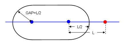
Рисунок 348: Рекомендуемый зазор при моделировании автоконтакта

Если длина стороны, L элемента меньше, чем GAP, самоконтакт будет даже вычислен с начала вычисления.

Такая ситуация может быть принята, если это исключение, но не для частых случаев в самоударном интерфейсе. Можно локализовать источник этого сообщения, используя препроцессор и выбирая элементы по критериям размера.

Разрыв

Когда моделируется разрыв и ожидается, что элементы выйдут из строя, важно иметь дело с вышедшими из строя элементами, определенными либо как основной сегмент, либо как вторичные узлы.

Когда элемент удаляется, соответствующий ему сегмент все равно учитывается, а его узлы все равно рассматриваются для контакта. Такое поведение может привести к огромной ошибке, поскольку удаленные элементы не имеют жесткости; поэтому рекомендуется установить флаг I_del на 2, когда ожидается отказ. Этот флаг удалит любой вышедший из строя элемент с основной поверхности, а соответствующие узлы будут удалены из списка вторичных узлов.

Интерфейс тянущихся стержней (/INTER/TYPE8)

Интерфейс TYPE8 используется для моделирования тянущихся стержней. Этот интерфейс в основном используется в обрабатывающей промышленности для моделирования формовки металла. тянущиеся стержни используются для предотвращения скольжения металлической полосы во время процесса штамповки.

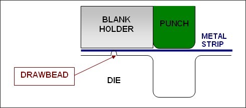
width

5.11394in

height

2.26014in

Рисунок 349: Процесс штамповки

Моделирование тянущихся стержней с использованием интерфейса TYPE8 заключается в определении линии вторичных узлов и основной поверхности. Набор вторичных узлов необходимо отсортировать, поскольку входная сила является силой на единицу длины, а длина вычисляется как расстояние между двумя последовательными вторичными узлами. Как только вторичный узел выступает на основную поверхность, ко всем основным узлам прикладывается касательная сила, противодействующая их касательной скорости (рис. 350). Следовательно, металлическая полоса не скользит.

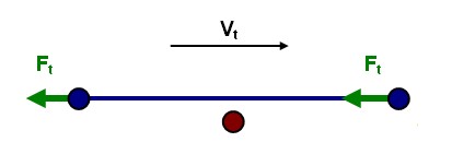
Рисунок 350: Сила натяжения

Примечание: Глобальная сила, действующая на основную поверхность не может быть больше силы натяжения на единицу длины (определяется пользователем), умноженной на расстояние двух последовательных вторичных узлов. В этом случае произойдет скольжение металлической полосы.

Распространенная проблема

В случае, если тяговый валик не является непрерывным, необходимо создать несколько интерфейсов TYPE8, по одному интерфейсу для каждого непрерывного тягового валика. В противном случае сила тягового валика может быть слишком высокой между двумя последовательными узлами, которые не являются частью одного и того же непрерывного тягового валика.

Рисунок 351 иллюстрирует этот момент. Серая часть может быть капотом автомобиля, и в процессе штамповки необходимы три тяговых валика. Если создается только один интерфейс TYPE8, поскольку тяговые валики не являются непрерывными, расстояние между узлами N17 и N18 намного больше, чем среднее расстояние между двумя последовательными узлами. Следовательно, сила тягового валика, приложенная к узлам N17 и N18, может быть слишком высокой, что приведет к нереалистичной деформации в этих областях.

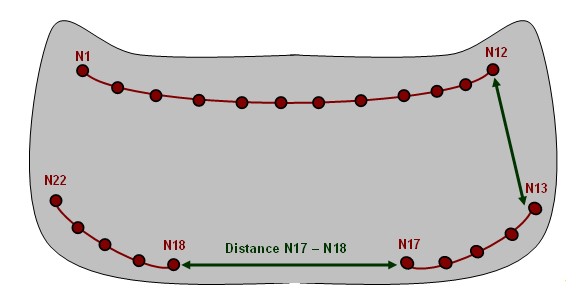
Рисунок 351: Пример штамповки капота

Интерфейс «край-к-краю» (/INTER/TYPE11)

Интерфейс TYPE11 используется для моделирования удара между линиями для одномерной сетки или кромками в оболочечных и сплошных сетках.

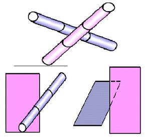
Рисунок 352: Контакт «край-к-краю»

В сочетании с интерфейсом TYPE7 интерфейс TYPE11 решает случаи блокировки и использует ту же формулировку штрафа и алгоритм поиска, что и интерфейс TYPE7.

Интерфейс TYPE 11 использует сложные математические алгоритмы; поэтому настоятельно рекомендуется использовать его только при необходимости. Огромный интерфейс TYPE11 может замедлить вычисления.

Квадратический контакт поверхности (/INTER/LAGMUL/TYPE16 и /INTER/LAGMUL/TYPE17)

Интерфейс TYPE16 позволяет определять условия контакта между группой узлов (вторичных) и кривой поверхностью квадратичных элементов (основной частью), как показано на рисунке 353 для симметричного контакта. Основная часть может быть изготовлена ​​из 16-узловых толстых оболочек или 20-узловых кирпичей. Метод множителей Лагранжа используется для применения условий контакта; поэтому не требуется применять зазор. Некоторые приложения этого интерфейса - скользящие контакты без зазоров, как в моделировании коробки передач.

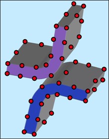
Рисунок 353: Интерфейс TYPE16 — Контакт узла с квадратичной поверхностью

Интерфейс TYPE17 позволяет моделировать контакт между двумя квадратичными поверхностями с использованием метода множителей Лагранжа. Это обобщенная форма интерфейса TYPE16, в котором контакт на двух квадратичных поверхностях решается напрямую. Предполагается, что контакт будет скользящим или связанным.

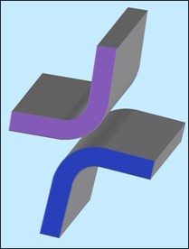
Рисунок 354: Интерфейс TYPE17 — квадратичная поверхность к квадратичной поверхности Контакт

Как определено выше, оба интерфейса не моделируют эффекты трения. Контакт рассматривается как связанный или без трения (чистое скольжение).

Примечание: При использовании интерфейсов с методом Лагранжа Множителя не рекомендуется симметрировать контакт.

Связанный интерфейс (/INTER/TYPE10)

Этот интерфейс похож на интерфейс TYPE7, за исключением жесткости, которая остается постоянной во время контакта.

Более того, после удара вторичный узел становится привязанным к основной поверхности с отскоком или без него (флаг \(I_{tied}\)).

Жесткость

Во время удара добавляется безмассовая пружина с постоянной жесткостью, чтобы оттолкнуть вторичный узел назад. Более того, когда вторичный узел завязывается, вторая безмассовая пружина используется для удержания вторичного узла близко к точке удара. В зависимости от того, допускается ли отскок, эти две пружины сохраняются, когда вторичный узел больше не проникает.

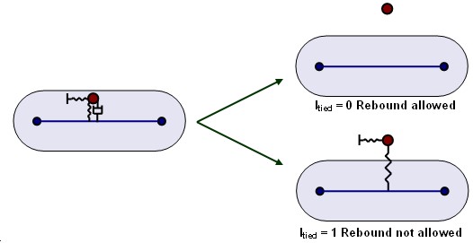
Рисунок 355: Интерфейс TYPE10

см так же

/INTER/TYPE10 (Starter)

Нагрузки

Предварительная нагрузка

Возможность предварительной нагрузки секции элементов доступна с помощью опции /PRELOAD. Это можно использовать для моделирования силы предварительного натяжения в болтах, используемых в сборках.

Натяжение болтов

Подробности физической проблемы натяжения болтов.

Типичная последовательность.

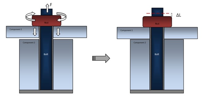
Рисунок 356: Предварительно напряженная сборка — приложение предварительных натяжных нагрузок (шаг 1)

На шаге 1, при предварительной сборке конструкции, гайки на соответствующих болтах затягиваются, как правило, с применением заданного крутящего момента (который преобразуется в заданную силу натяжения в соответствии с шагом резьбы).

В результате рабочая часть болта становится короче на расстояние \(\Delta L\). Это расстояние зависит от приложенной силы, податливости болта и предварительно натянутой сборки.

С точки зрения анализа FEA важно признать, что:

• Предварительное натяжение укорачивает рабочую часть болта, удаляя определенную длину болта из активной конструкции (в действительности этот сегмент скользит через гайку, но чистый эффект — это сокращение рабочей длины болта). Поскольку болт растягивается, эффективная длина материала болта для покрытия расстояния от крепления болта до гайки становится меньше

• Расчет укорочения каждого болта \(\Delta L\) из-за приложенных сил f требует решения FEA всей модели с приложенными силами предварительного натяжения. Это связано с тем, что величина перемещения гайки из-за данной силы зависит от податливости болтов, узла, который скрепляется болтами, а также зависит от перекрестного взаимодействия между несколькими предварительно натянутыми болтами.

В конце шага 1 величина укорочения \(\Delta L\) для каждого болта устанавливается и «блокируется», просто оставляя гайки в положении, которого они достигли на этапе предварительного натяжения.

На этапе 2, с укорочением \(\Delta L\) всех болтов «заблокированных», другие нагрузки прилагаются к сборке (рисунок 357). На этом этапе напряжения и деформации в болтах обычно будут меняться, в то время как длина удаленного материала \(\Delta L\) остается постоянной для каждого болта.

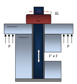
Рисунок 357: Предварительно натянутая сборка — приложение рабочих нагрузок с «заблокированным» укорочением болта (шаг 2)

Определение предварительной нагрузки

Чтобы создать предварительную нагрузку в болте, сначала используется опция раздела /SECT для определения набора элементов, к которым будет применена предварительная нагрузка.

Затем идентификатор раздела ссылается на вход /PRELOAD. Для создания предварительной нагрузки начальное растягивающее напряжение, приложенное к набору элементов, указанных в сечении, приводит к сокращению длины болта в локальной оси z определенного /SECT.

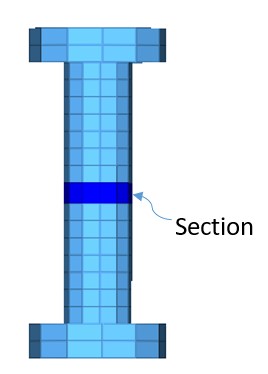
Рисунок 358: Раздел, определяющий группу элементов для предварительной нагрузки

Величина предварительной нагрузки может быть введена как сила (по умолчанию) или напряжение в зависимости от опции ввода /PRELOAD, \(I_{typ}\). Если введена сила, начальная площадь поперечного сечения /SECT используется для расчета напряжения, которое применяется для создания предварительной нагрузки. В заданное время /PRELOAD \(T_{start}\) жесткость материала элементов, определенных в разделе, уменьшается, и растягивающее напряжение применяется к определенным элементам сечения, что приводит к уменьшению длины элементов, что приводит к требуемой предварительной нагрузке. Поскольку жесткость материала уменьшается, количество деформации, создаваемой в элементе, также уменьшается.

Время предварительной нагрузки между \(T_{start}\) и \(T_{stop}\) - это время, когда жесткость материала возвращается от пониженной жесткости к исходной жесткости материала. Как показано на рисунке 359, есть постоянная пониженная жесткость, затем линейное увеличение жесткости до исходной жесткости материала, за которой следует постоянная жесткость.

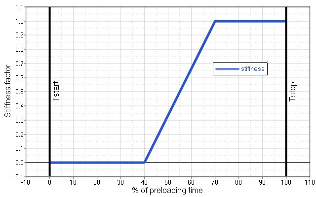
Рисунок 359: Увеличение жесткости материала

Предварительная нагрузка также может быть активирована с помощью /SENSOR, и в этом случае

\(T_{start}\) и \(T_{stop}\) времена смещаются на основе времени активации датчика.

Для вывода силы предварительного натяжения секции следует создать /TH/SECTIO. В зависимости от скрепляемой сборки, зазора контакта между деталями болта и материала болта, ввод предварительного натяжения болта может не совпадать с выходной силой секции.

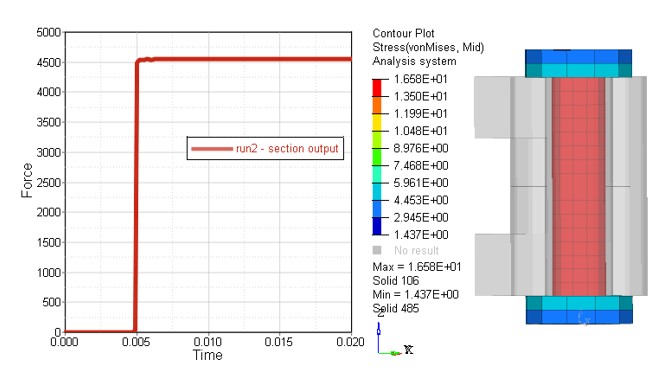
Рисунок 360: Выход сечения и напряжение болта

Подушки безопасности моделируются как контролируемые объемы /MONVOL несколькими различными способами.

Существуют и другие типы контролируемых объемов, используемые для моделирования закрытых объемов, заполненных газом или жидкостью, таких как: шины, газовые баллоны (плеск игнорируется) и ЖК-экраны.

Контролируемый объем (/MONVOL)

Контролируемый объем определяется одной или несколькими частями оболочки (3-узловыми или 4-узловыми).

Определенная поверхность должна быть замкнутой (PRADIOS Starter проверяет ее и выводит сообщение об ошибке, если поверхность не замкнута). Нормаль оболочек должна быть ориентирована вне объема. Можно обратить нормаль оболочек для заданной детали, задав отрицательный номер детали (или используя соответствующий препроцессор, чтобы обратить их).

Следующие типы контролируемого объема могут использоваться для моделирования подушек безопасности:

• AIRBAG1: классическая подушка безопасности с равномерным давлением

• AREA: замкнутая поверхность для вывода ее объема и области постобработки

• COMMU1: камеры с равномерным давлением со связью

• FVMBAG1: подушка безопасности с неравномерным давлением, решенная методом конечных объемов

• GAS: используется для моделирования давления в шинах или простого топливного бака

• LFLUID: линейный контролируемый объем жидкости для моделирования несжимаемой жидкости

• PRES: простой контролируемый объем с равномерным давлением

Свойства и законы материала, используемые для моделирования ткани, могут быть:

• /MAT/LAW19 + /PROP/SH_ORTH - Используется для моделирования ткани с линейным упругим поведением.

• /MAT/LAW58 + /PROP/SH_FABR - Используется для моделирования поведения нелинейной упругой ткани.

Рекомендации:

• Материалы ткани ведут себя как мембрана, поэтому рекомендуется использовать одну точку интегрирования по толщине, N=1.

• Ткань можно смоделировать с помощью элемента оболочки с 3 узлами, используя формулировку элемента стандартного треугольника (C0) по умолчанию, которая не имеет песочных часов, или с помощью оболочки с 4 узлами, используя элемент QBAT, \(I_{shell}\) =12 с \(I_{smstr}\) =11.

• Хотя больше не рекомендуется, если используется \(I_{shell}\) =4, то, чтобы избежать песочных часов, определите коэффициент песочных часов мембраны оболочки hm и песочные часы оболочки из плоскости hf равными 10%.

• Чтобы определить сообщающуюся поверхность для контролируемого объема типа COMMU1, следует использовать материалы пустот и свойства /MAT/VOID и /PROP/VOID).

• Тип FVMBAG1 может использоваться для моделирования эффектов потока газа, что необходимо при моделировании шторных подушек безопасности и симуляций Out Of Position (OOP).

• Обычно для определения контакта самоудара интерфейса можно определить один интерфейс самоудара TYPE7 и один контакт интерфейса край-в-край TYPE11.

Если есть несколько начальных проникновений, установите Inacti =6. Эти два контакта также можно заменить одним контактом TYPE19.

AIRBAG1

Предполагается равномерное давление внутри объема. Предполагается идеальный газовый закон и адиабатические условия. Впрыскиваемая масса (или массовый расход) и температура определяются как функция времени с использованием свойства инжектора. Датчик может определять время запуска инфлятора.

Сдувание вентиляционного отверстия происходит после достижения критерия давления (\(P_{def}\)) или времени (\(t_{def}\)).

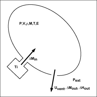
Рисунок 361:

Численное демпфирование

Вязкость может использоваться для уменьшения числовых колебаний.

Если \(\mu\) =1, используется критическое демпфирование (масса оболочки и объемная жесткость). Вязкое давление, q вычисляется как: \(q=-\frac{\mu}{A}\sqrt{\frac{PA\rho t}{V}} \frac{dV}{dt}if\frac{dV}{dt}<0\)

\(q=0 if \frac{dV}{dt}>0\)

Где,

\(t\) Толщина ткани

\(\rho\) Судьба ткани

\(A\) Поверхность мешка

Приложенное давление:

\[P-P_{ext}+q \tag{240}\]

Начальные условия

Чтобы избежать начального неравновесия и математического разрыва для нулевой массы или нулевого объема, следующие начальные условия задаются в нулевой момент времени (\(I_{equil}\) =0) или в начале струйной подачи (если \(I_{equil}\) =1).

• \(P_{ext}=P_{ini}\) внешнее давление

• \(T_{0}=T_{ini}\) начальная температура (по умолчанию 295K)

• Если начальный объем меньше \(10^{-4}A^{3/2}\), добавляется постоянный малый объем для получения начального объема: \(V_{ini}=10^{-4}A^{3/2}\)

• Начальная масса, энергия и плотность определяются из приведенных выше значений.

Нет необходимости определять инжектируемую массу в нулевой момент времени.

Определение газов

1. Начальный и впрыскиваемый газ определяется с помощью /MAT/GAS. Можно определить четыре типа газа (MASS, MOLE, PREDEF или CSTA).

2. Тогда удельная емкость на единицу массы при постоянном давлении для газа равна:

• Тип МАССЫ

\[ \begin{align}\begin{aligned}C_{p}=\left(C_{pa}+C_{pb}T+C_{pc}T^{2}+C_{pd}T^{3}+\frac{C_{pe}}{T^{2}}+C_{pf}T^{4}\right) \tag{241}\\- Тип МОЛЬ\end{aligned}\end{align} \]

\[C_{p}=\frac{1}{MW}\left(C_{pa}+C_{pb}T+C_{pc}T^{2}+C_{pd}T^{3}+\frac{C_{pe}}{T^{2}}\right)\tag{242}\]

Где MW — молекулярная масса газа.

• Тип CSTA

Пользовательский ввод \(C_{p}\) и \(C_{V}\) с единицей \(\left[\frac{J}{kgK}\right]\).

• Тип PREDEF

Около 14 часто используемых газов (N2, O2, воздух и т. д.), предопределенных в PRADIOS.

2. Впрыскиваемый газ

   \(N_{jet}\) определяет количество инжекторов по контролируемому

   объему. Материал инжектора определяется с помощью /MAT/GAS. Свойства инжектора (/PROP/INJECT1 или /PROP/INJECT2) определяют кривую инжектируемой массы, определенную \(fct\_ID_{M}\), и кривую инжектируемой температуры, определенную \(fct\_ID_{T}\).

   Можно получить кривую массы впрыска и температуру впрыска:

   • От производителя подушек безопасности

   • Из теста бака

sens_ID — это номер датчика для начала впрыска.

3. Эффект струи \(I_{jet}\) используется только для /MONVOL/AIRBAG1 or ``/MONVOL/COMMU1 ``

   Если \(I_{jet}\neq 0\), эффект струи моделируется как избыточное давление \(\Delta P_{jet}\), приложенное к элементам мешка.

\[\Delta P_{jet}=\Delta\text{P}(t)\cdot\Delta\text{P}(\theta)\cdot\Delta\text{P}(\delta)\cdot\max(\mathbf{n}\cdot\mathbf{m},0) \tag{243}\]

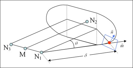
Рисунок 362:

N₁, N₂ и N₃ определяются на основе геометрии инжектора (см. Руководство по вводу PRADIOS Starter)

\(\Delta P(t),\Delta P(\theta),\Delta P(\delta)\) являются эмпирическими функциями, предоставляемыми пользователем через \(fct\_ID_{Pt},fct\_ID_{P\theta\)}` и \(fct\_ID_{P\delta}\)

Определение вентиляционного отверстия

\(N_{vent}\) определяет количество используемых вентиляционных отверстий.

\(sur f\_ID_{v}\) — идентификатор поверхности, определяющий вентиляционное отверстие

\(A_{vent}\) — площадь вентиляционного отверстия (если \(sur f\_ID_{v}\) = 0) или масштабный коэффициент (\(sur f\_ID_{v}\neq 0)\)

\(B_{vent}\) = 0 (если \(surf\_ID_{v} = 0)\) или масштабный коэффициент на поверхности воздействия (\(surf\_ID_{v}\neq 0)\)

\(T_{stop}\) — время остановки вентилирования

\(T_{start}\) — время начала утечки

\(\Delta P_{def}\) — относительное давление дефляции вентиля

\(\Delta tP_{def}\) — продолжительность времени в течение которого \(\Delta P>\Delta P_{def}\)

\(fct\_ID_{v}\) — идентификатор функции \(f_{p}(P-P_{ext})\) для модели Чемкина (\(I_{form}=2)\)

\[vent\_holes\_surface=A_{vent}\cdot A_{nom_impacted}\cdot f_{p}(I)\cdot f_{p}(P-P_{ext})\cdot f_{p}\left(\frac{A_{nom\_impacted}}{A_{0}}\right)\tag{244}\]

Если \(fct\_ID_{v}\neq 0\), скорость оттока, v определяется Чемкиным как:

\[v=Fscale_{v}f_{v}(P-P_{ext}) \tag{245}\]

Где, \(Fscale_{v}\) — масштабный коэффициент функции \(fct\_ID_{v}\).

а исходящая масса вычисляется как: .. math:: dot{m}_{out}=rhocdot A_{vent}cdotmathsf{f}_{v}big{(}P-P_{ext}big{)}cdot FScal_{v}tag{246}

Или, с сохранением энтальпии между подушкой безопасности и вентиляционным отверстием, адиабатическими условиями и безударной струей, можно выразить исходящий массовый поток через вентиляционные отверстия как функцию \(P_{ext}\rho, P_{vent}, u_{vent}\) и \(A_{vent}\).

\[\dot{m}_{out}=\rho_{vent}\cdot A_{vent}\cdot u=\rho\bigg{(}\frac{P_{ext}}{P}\bigg{)}^{\frac{1}{\gamma}}\cdot A_{vent}\cdot u\tag{247}\]

В случае сверхзвукового выходного потока давление на выходе, \(P_{vent}\) равно внешнему давлению, \(P_{ext}\) для потока без скачков уплотнения. Для потока с скачками уплотнения,

\(P_{vent}\) равно критическому давлению, \(P_{crit}\), а скорость, u ограничена критической скоростью звука:

\[u^{2}<\frac{2}{\gamma+1}c_{2}=\frac{2\gamma}{\gamma+1}\frac{P}{\rho}\tag{248}\]

и

\[P_{crit}=P\bigg{(}\frac{2}{\gamma+1}\bigg{)}^{\frac{\gamma}{\gamma+1}}\tag{249}\]

\[P_{vent}=\max(P_{crit} P_{ext})\tag{250}\]

Исходящий массовый поток газа i равен:

\[\dot{m}_{out}(i)=\frac{V^{(i)}}{V}\dot{m}_{out}\tag{251}\]

Где, \(V^{(i)}\) is the volume occupied by gas i и satisfies:

\[V^{(i)}=\frac{\dot{n}(i)}{n}V \tag{252}\]

для \(PV^{(i)}=\dot{n}(i)RT\) и \(PV=\left[\sum_{i}\dot{n}(i)\right]RT\).

Далее,

\[\dot{m}_{out}(i)=\frac{\dot{n}(i)}{\dot{n}(i)}\dot{m}_{out}\tag{253}\]

Пористость

Изоэнтальпическая модель также используется для пористости. В этом случае можно определить поверхность для исходящего потока:

\[A_{eff}=C_{ps}\cdot Area_{ps} \tag{254}\]

или .. math:: A_{eff}=mathrm{C}_{ps}(t)cdot Area_{ps}(P-P_{ext})

Где,

\(C_{ps}(t)\) Функция \(fct\_ID_{cps}\)

\(Area_{ps}(P-P_{ext})\) Функция \(fct\_ID_{aps}\)

Также можно определить закрытие пористой поверхности при возникновении контактов, определив опцию интерфейса \(I_{bag}\) =1.

см также

Контролируемый объем (теоретическое руководство)

COMMU1

Эта опция используется для имитации камерных подушек безопасности и может использоваться для раскрытия подушки безопасности.

Каждый контролируемый объем типа COMMU1 работает как контролируемый объем типа AIRBAG1 с возможной вентиляционной связью с некоторым другим контролируемым объемом типа COMMU1. Таким образом, камерная подушка безопасности разработана с двумя или более контролируемыми объемами типа COMMU1.

Каждый контролируемый объем может иметь нагнетатель и вентиляционные отверстия.Case 1: Folded Airbag

Для моделирования сложенной подушки безопасности используется один контролируемый объем типа COMMU1 для каждой сложенной части. Граница между двумя сложенными частями закрыта набором свойств пустоты (фиктивным). Область сообщения определяется этим набором свойств пустоты. Давление в каждой сложенной части будет разным, а область сообщения будет увеличиваться во время надувания. При таком моделировании объем с инфлятором будет надуваться первым и перед сложенными частями.

Том 1

Предложение 1 + 4 + 5: Коммуникационная область: том 1 по 2: предложение 4 том 1 по 3: предложение 5

Том 2

Предложение 2 + 4: Коммуникационная область: том 2 по 1: предложение 4

Том 3

Предложение 3 + 5: Коммуникационная область: том 3 по 1: предложение 5

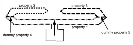
Рисунок 363:

Случай 2: Общее использование

Контролируемый объем 1 может сообщаться с контролируемым объемом 2 с или без связи от 2 к 1. Коммуникационная область, давление дефляции или время от 1 к 2 могут отличаться от соответствующих значений от 2 к 1. Таким образом, можно смоделировать коммуникацию клапана.

Два коммуникационных контролируемых объема могут иметь общие узлы или общий набор свойств оболочки, но это необязательно.

Объем 1 сообщается с объемом 2, а объем 2 с объемами 1 и 3, но нет связи от 3 к 2.

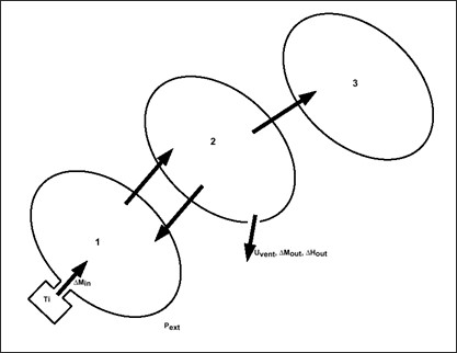
Рисунок 364:

Общие уравнения

Используются те же уравнения для контролируемого объема типа AIRBAG1, но входящая и исходящая энтальпия и кинетическая энергия будут учитывать сообщающиеся мешки. Для каждого сообщающегося объема, для которого давление ниже, чем в текущем объеме, поток массы и энергии вычисляется с теми же уравнениями для вентиляционных отверстий, внешнее давление просто заменяется давлением сообщающегося объема:

\[u^{2}=\frac{2\gamma}{\gamma-1}\frac{P}{\rho}\Bigg{(}1-\Big{(}\frac{P_{vent}}{P}\Big{)}^{\frac{\gamma-1}{\gamma}}\Bigg{)}\tag{256}\]

с,

\[P_{vent}=\max\Big{(}P_{crip} P_{neighbor}\Big{)}\tag{257}\]

\[\rho_{vent}=\Big{(}\frac{P_{vent}}{P}\Big{)}1\Big{/}\gamma \tag{258}\]

\[\dot{m}_{out}=\rho_{vent}\cdot A_{vent}\cdot u=\beta\Big{(}\frac{P_{ext}}{P}\Big{)}^{\frac{1}{V}}\cdot A_{vent}\cdot u\tag{259}\]

\[\dot{E}_{out}=m_{out}\frac{E}{\rho V}=\Big{(}\frac{P_{ext}}{P}\Big{)}^{\frac{1}{V}}A_{vent}u\frac{E}{V}\tag{260}\]

Эти потоки массы и энергии удаляются из текущего объема и добавляются к сообщающемуся объему в следующем цикле.

Нагнетатель, вентиляционное отверстие, начальные условия

Нагнетатель, атмосферные вентиляционные отверстия и начальные условия идентичны контролируемому объему типа /MONVOL/AIRBAG1.

Удельный вход

Конкретный ввод для этого типа:

\(\mu\) — коэффициент вязкости

\(P_{ext}\) — внешнее давление

\(\Delta P_{def}\) — относительное давление дефляции вентиляционного отверстия

\(A_{vent}\) — площадь дефляции (\(surf\_ID_{v}=0)\) или коэффициент расхода (\(surf\_ID_{v}\neq 0\))

\(T_{start}\) — время дефляции вентиляционного отверстия

Начальный газ и впрыскиваемый газ определяются с помощью /MAT/GAS.

Свойства впрыска определяются с помощью /PROP/INJECT1 или /PROP/INJECT2.

\(fct\_ID_{M}\) — кривая массы впрыска (или массовая скорость)

\(Fscale_{M}\) — масштабный коэффициент для кривой массы впрыска (или массовой скорости)

\(fct\_ID_{T}\) — кривая температуры впрыска \(Fscale_{T}\) масштабный коэффициент для кривой температуры впрыска

sens_ID — номер датчика для начала впрыска

Nvent — номер вентиляционного отверстия

Nbag — номер сообщающегося объема

Для каждого сообщающегося объема (от 1 до Nbag):

bag_ID — идентификация сообщающегося объема

\(surf\_ID_{c}\) определяет область связи

\(\Delta P_{Cdef}\) — относительное давление дефляции

\(A_{com}\) — область связи (\(surf\_ID_{c}=0)\) или коэффициент разряда (\(surf\_ID_{c}\neq 0)\)

\(T_{com}\) время сдувания области связи

В объеме j входные данные для связи с объемом k касаются только потока от j до k. Данные, касающиеся потока от k до j, определены во входном объеме k.

См. также

Контролируемый объем (теоретическое руководство)

FVMBAG1

Предполагается неравномерное давление внутри объема. Поток газа в FVMBAG1 решается с использованием схемы интегрирования конечного объема, которая позволяет корректно моделировать поток газа через подушку безопасности.

Поскольку поток газа смоделирован, поведение развертывания и раскрытия является правильным, что необходимо для моделирования пассажира вне положения и раскрытия подушек безопасности занавесок.

Предполагаются идеальный газовый закон и адиабатические условия. Впрыскиваемая масса, скорость и температура определяются как функция времени. Впрыскиваемая скорость получается с помощью:

\[v_{in}(t)=\frac{dm(t)/dt}{S\rho_{in}(t)}\]

Где, S - поверхность инжектора.

Датчик может определять время запуска инфлятора.

Дефляция вентиляционного отверстия доступна после достижения критерия давления (\(P_{def}\)) или времени (\(t_{def}\)).

В этой версии теплоемкость газа \(C_{p}\) предполагается постоянной.

Более подробную информацию см. в Руководстве по моделированию подушек безопасности FVMBAG1.

ГАЗ

Этот контролируемый объем обычно используется для моделирования давления в шинах или простого топливного бака.

Для модели шин \(V_{i}\) равно нулю, а для топливного бака \(V_{i}\) — объем топлива.

Примеры /MONVOL/GAS

• Модель шины:

Входные данные:

◦ \(y = 1.4\)

◦ \(\mu\)

◦ \(P_{ext} = 10^{5}\) Pa

◦ \(P_{ini}\) = начальное давление в шинах

Тогда давление в шине равно \(P_{tire} = P_{ini} - P_{ext}\)

◦ \(V_{inc} = 0\)

• Модель топливного бака, если пренебречь эффектом плескания

  Только если пренебречь эффектом плескания, давление в частично заполненном топливном баке можно смоделировать с типом ГАЗ, контролируемым объемом. Используйте следующие входные данные:

◦ \(y = 1.4\)

◦ \(\mu\)

◦ \(P_{ext} = 10^{5}\) Pa

◦ \(P_{ini} = 10^{5}\) Pa

◦ \(V_{inc}\) = volume of fuel

см также

GAS Type

LFLUID

Линейный контролируемый объем жидкости, который моделирует объем, заполненный жидкостью.

В контролируемом объеме LFLUID определяются плотность и объемный модуль жидкости. Существуют дополнительные кривые для определения массового расхода в и из с течением времени. Объемный модуль также может быть определен как функция времени.

Дополнительное давление может быть включено путем определения функции для давления, добавленного в зависимости от времени. Наконец, можно определить максимальное давление в объеме.

PRES

Простой контролируемый объем идеального газа, где относительное давление является функцией относительного объема или функцией времени.

В контролируемом объеме PRES относительное давление определяется как \(P_{rel}\) = давление внутри контролируемого объема - атмосферное давление.

Относительное давление определяется с помощью функции одним из двух способов. По умолчанию относительное давление определяется как функция относительного объема \(P_{rel}\frac{V_{o}}{V}\), или давление может быть функцией времени \(P_{rel}(t)\).

См. также

Тип PRES

Временной шаг контролируемого объема————-

Шаг времени «AIRBAG1» оценивается в двигателе, но этот шаг времени никогда не будет контролировать шаг времени во время выполнения. Если это так, то это означает, что в колоде ввода есть нефизическое определение подушки безопасности.

Элемент управления шагом времени

/DT/AIRBAG

Определяет \(\Delta T_{sca}\) и \(\Delta T_{min}\) для подушек безопасности

\(\Delta T_{sca}\Delta T_{min}\)

/DT/FVMBAG

Определяет \(\Delta T_{sca}\) и \(\Delta T_{min}\) для подушки безопасности с конечным объемом

\(\Delta T_{sca}\Delta T_{min}\)

/DT/FVMBAG используется только для контролируемых объемов типа /MONVOL/FVMBAG1. \(\Delta T_{sca}\Delta T_{min}\) можно определить для обеспечения стабильности и минимального размера шага времени, вызывая дополнительные слияния конечных объемов, когда сущность FVMBAG1 штрафует вычисления. /DT/FVMBAG/1 используется для слияния конечных объемов, когда \(dt<\Delta T_{min}\).

Руководство по моделированию подушек безопасности FVMBAG1

Область применения

Настоящие руководящие принципы определяют требования к моделированию и проверке для численных моделей подушек безопасности в PRADIOS с методом конечного объема (FVM).

Эти руководящие принципы основаны на производственных версиях PRADIOS 2017.2.5, 2019.2.4, 2020.1, 2021.2 двойной точности, которые используются многими производителями подушек безопасности. Версия PRADIOS с одинарной точностью не может использоваться для расчетов подушек безопасности. Требования руководящих принципов основаны на общепринятой практике моделирования подушек безопасности. Некоторые из требований не связаны напрямую с FVM, но рекомендуются для создания модели подушки безопасности, которую легко понять и включить в моделирование столкновений.

• FVM - Метод конечного объема

• FV - Конечный объем

• UP - Равномерное давление

Общие требования к моделям подушек безопасности

Численные модели подушек безопасности создаются для численного моделирования событий аварий, связанных с проблемами безопасности пассажиров. Модели подушек безопасности могут отличаться по количеству деталей и точности в зависимости от их предполагаемого применения.

Модель подушки безопасности должна обладать всеми типичными характеристиками оборудования подушек безопасности: газогенератор, корпус, фиксаторы, межкамерные компоненты, вентиляционные отверстия, определение ткани с покрытием, пористость ткани для ткани без покрытия, ремни, швы и т. д.

Геометрия, масса, инерционные свойства и материалы модели подушки безопасности должны соответствовать данным оборудования и САПР.

Различные части подушки безопасности, такие как компоненты подушки безопасности, внешние поверхности, внутренние поверхности и вентиляционные отверстия, должны быть организованы в сборки /SUBSET.

Каждая модель подушки безопасности должна представлять собой модель, которая будет работать независимо и использоваться в других компонентах или полных моделях автомобиля в качестве включаемых файлов.

Модель подушки безопасности должна быть предоставлена ​​в проектном положении. Размещение подушки безопасности внутри модели компонента или полной модели автомобиля должно быть выполнено с использованием карт /TRANSFORM.

Сетка и складывание

Ткань подушки безопасности должна быть сеткой в ​​несложенном состоянии с использованием триа элементов со средним размером элемента от 3 до 4 мм. Смешанная + триа сетка разрешена, начиная с версии 2021.2. Более крупные размеры элементов приемлемы только для вентиляционных отверстий и других компонентов, которые используют материал пустоты (например, межкамерный компонент пустоты). Все узлы элементов, связанных с пустотами, должны быть прикреплены к окружающим компонентам ткани. Ткани подушки безопасности имеют низкий модуль упругости, и поэтому обычно размер элементов не влияет на временной шаг.

Внешние компоненты ткани подушки безопасности должны образовывать замкнутый объем с нормальными векторами, направленными наружу.

Примечание: Это ограничение было выпущено в версии 2021, но по-прежнему рекомендуется иметь внешнюю нормаль.

Пересечения между любыми компонентами подушки безопасности (например, внешними, внутренними, инфлятором или корпусом) не допускаются.

Складывание подушки безопасности должно выполняться с использованием предварительного моделирования в соответствии с проектом складывания САПР. Модель складывания должна использовать проверенные определения и контакты материала ткани. PRADIOS является предпочтительным решателем для предварительного моделирования складывания (решения для подушек безопасности). Это гарантирует, что сложенная модель будет работать правильно с определением внутреннего контакта подушки безопасности, перечисленным в соответствующих разделах.

Справочная геометрия

Справочная геометрия должна быть представлена ​​как геометрия на основе плоских узлов (/XREF) или элементов (/EREF).

В /EREF части опорной геометрии подушки безопасности могут быть отдельными частями, которые не соединены.

В некоторых случаях /XREF также может использоваться для опорной геометрии, которая не соединена. В этом случае каждая часть, указанная в карте, не должна соединяться сама с собой в фактической модели подушки безопасности.

Опорная геометрия должна быть параллельна глобальной плоскости XY.

Примечание: Это не является требованием подхода FVM, но вместо этого упрощает определение ортотропных направлений компонентов подушки безопасности.

Для эталонной геометрии, представляющей собой замкнутый объем:

• геометрический центр не сложенной подушки безопасности должен находиться в точке X=0, Y=0 или Z=0

• нормальные направления компонентов в опорной геометрии должны быть такими же, как в сложенной модели подушки безопасности

• пересечения не допускаются в развернутой опорной геометрии подушки безопасности

Для разъединенной опорной геометрии подушки безопасности на основе элементов /EREF:

• каждый компонент должен находиться в плоскости Z=0

• нормальные направления компонентов в опорной геометрии должны быть такими же, как в сложенной модели подушки безопасности

В ходе итераций проектирования эталонная геометрия может быть изменена или трансформирована с целью исследования влияния незначительных изменений формы подушки безопасности на ее характеристики.

Примечание: При использовании опорной геометрии временной шаг для ткани рассчитывается на основе размера опорной геометрии элементов. Исходные направления анизотропии материала также рассчитываются на основе опорной геометрии.

Газовый генератор

Модель газогенератора должна представлять все детали, доступные в данных САПР: газогенератор, отверстия инжектора и фиксаторы.

Модель газогенератора должна представлять все детали, доступные в данных САПР: газогенератор, отверстия инжектора и фиксаторы. Отверстие инжектора представлено элементами на поверхности инфлятора. Компоненты инфлятора моделируются как компонент оболочки с материалом LAW2 и пауком жесткого тела /RBODY. Массовые и инерционные свойства компонентов инфлятора должны соответствовать оборудованию.

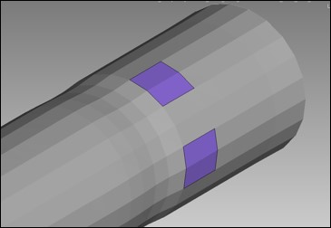
Рисунок 365: Элементы инфлятора и инжектора

Направление впрыска противоположно нормали элемента. Элементы разных инжекторов не должны иметь общих элементов. PRADIOS предположит, что элемент принадлежит последнему определенному инжектору.

Элементы из вентиляционного отверстия или пористой поверхности также не должны иметь общих элементов с инжекторами. PRADIOS автоматически исключает элементы из определения вентиляционной или пористой поверхности.

Поверхность инжектора также может быть определена на внутренней поверхности внутри объема подушки безопасности. В этом случае направление потока газа противоположно нормали элемента внутренней поверхности.

Свойства инфлятора /PROP/INJECT1 и /PROP/INJECT2 определяют параметры состава впрыскиваемого газа. Каждый из газовых компонентов должен быть указан как отдельная карта материала: /MAT/GAS/MASS, /MAT/GAS/MOLE или /MAT/GAS/PREDEF. В последнем случае материал газа создается в соответствии с ключевым словом, указанным в карте /MAT/GAS/PREDEF, и единицами, указанными в карте /BEGIN.

Пример определения материала газа в кг, мм, мс (предопределено, связано с массой, связано с молем):

#---1----|----2----|----3----|----4----|----5----|----6----|----7----|----8----|----9----|---10----|
/MAT/GAS/MASS/1
INJECTOR MIXTURE
#                           MW
                       .03300
#                         Cpa        Cpb          Cpc          Cpd          Cpe
                       1070.00        0            0            0            0
#                         Cpf
                           0
#---1----|----2----|----3----|----4----|----5----|----6----|----7----|----8----|----9----|---10----|

Молекулярный вес и коэффициенты удельной теплоемкости определяются для каждого из компонентов впрыскиваемого газа.

Функция теплоемкости.

\[C_{p}=\left(C_{pa}+C_{pb}T+C_{pc}T^{2}+C_{pd}T^{3}+\frac{C_{pe}}{T^{2}}+P_{pf}T^{4}\right)\tag{262}\]

должна быть монотонно возрастающей для температур между температурой окружающей среды и максимальным значением температуры, указанным в температурных кривых инжектора. Если функция не монотонно возрастает, PRADIOS автоматически корректирует функцию \(C_{p}(T)\), чтобы сохранить ее монотонной. Это может произойти, когда \(C_{pe} > 0\) или один из \(C_{pb}, C_{pc}, C_{pd}, C_{pf}\) коэффициентов отрицательный.

Состав впрыскиваемого газа, массовый расход впрыскиваемого газа и температура для каждого из газовых компонентов определяются в картах /PROP/INJECT1 или /PROP/INJECT2.

Пример определения свойств инжектора:

#---1----|----2----|----3----|----4----|----5----|----6----|----7----|----8----|----9----|---10----|
/PROP/INJECT1/1
Inflator 1
#    Ngases      Iflow       Ascale_T
         5           1              1
#    mat_ID    fct_IDM        fct_IDT             Fscale_M             Fscale_T
         1           2              1                    0                   0
#    mat_ID    fct_IDM        fct_IDT             Fscale_M             Fscale_T
         2           3              1                    0                   0
#    mat_ID    fct_IDM        fct_IDT             Fscale_M             Fscale_T
         3           4              1                    0                   0
#    mat_ID    fct_IDM        fct_IDT             Fscale_M             Fscale_T
         4           5              1                    0                   0
#    mat_ID    fct_IDM        fct_IDT             Fscale_M             Fscale_T
         5           6              1                    0                   0
#---1----|----2----|----3----|----4----|----5----|----6----|----7----|----8----|----9----|---10----|

Эта карта затем ссылается на карту подушки безопасности /MONVOL/FVMBAG1.

Время срабатывания инжектора (TTF) должно определяться с помощью датчика в /MONVOL/FVMBAG1, а не с помощью смещения кривых массы и температуры.

Когда нагнетатель определен правильно и ссылается на /MONVOL/FVMBAG1, стартер PRADIOS выводит список элементов, используемых в качестве поверхности инжектора.

ELEM:  92 <-> SH3N : 55261587 - INFLATOR : 1
ELEM: 502 <-> SH3N : 55262048 - INFLATOR : 1
ELEM: 622 <-> SH3N : 55261581 - INFLATOR : 1
ELEM: 627 <-> SH3N : 55261568 - INFLATOR : 1
ELEM: 633 <-> SH3N : 55262068 - INFLATOR : 1
ELEM: 814 <-> SH3N : 55261601 - INFLATOR : 1

Модель инфлятора должна быть проверена с использованием моделирования испытания резервуара. Отчет об испытании резервуара должен включать давление и температуру, измеренные в ходе испытания, массовый расход инжектора для каждого из газовых компонентов и температурные кривые. Давление и температуру из испытания можно сравнить со средним давлением и температурой в моделировании.

Исходный воздух внутри подушки безопасности

Материал для воздуха внутри подушки безопасности должен быть указан либо через /MAT/GAS/MASS, /MAT/GAS/MOLE или /MAT/GAS/PREDEF.

В последнем случае материал газа определяется в карте /MAT/GAS/PREDEF в единицах, определенных в карте /BEGIN.

Общая карта материала для воздуха (кг, мм, мс):

#---1----|----2----|----3----|----4----|----5----|----6----|----7----|----8----|----9----|---10----|
/MAT/GAS/PREDEF/4
Initial gas
AIR
#---1----|----2----|----3----|----4----|----5----|----6----|----7----|----8----|----9----|---10----|
/MAT/GAS/MASS/102
AIR, kg, mm, ms
#                 MW
#                Cpa               Cpb                  Cpc                  Cpd                  Cpe
              966.99                0                    0                     0                   0
#                Cpf
                   0
#---1----|----2----|----3----|----4----|----5----|----6----|----7----|----8----|----9----|---10----|
/MAT/GAS/MOLE/104
AIR, kg, mm, ms
#                 MW
              0.028013
#                cpa               cpb                  cpc                  cpd                  cpe
               27.088               0                    0                    0                    0
#                cpf
                   0
#---1----|----2----|----3----|----4----|----5----|----6----|----7----|----8----|----9----|---10----|

Тот же материал воздуха, который используется в подушке безопасности, следует также использовать в качестве воздуха в моделировании испытания бака для проверки инжектора.

Материал ткани подушки безопасности

Нелинейный анизотропный материал LAW58, используемый в качестве материала подушки безопасности.

Материал должен быть испытан и проверен с помощью следующих испытаний: испытание на рамку изображения, испытание на двуосное растяжение и испытание на одноосное растяжение в направлениях утка и обмотки.

Испытание на рамку изображения определяет поведение материала ткани при сдвиге.

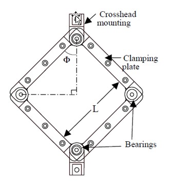
Рисунок 366: Установка для сдвига рамки картины

Напряжение сдвига как функция угла анизотропии в градусах следует извлечь из кривых смещения силы из теста рамки картины и использовать в качестве входной кривой в материале LAW58.

Где, \(\alpha=\left(\frac{\pi}{2}\right)-2\cdot\arccos\left(\frac{1}{\sqrt{2}}-\frac{D}{L}\right)\text{and}D\)

Вертикальное смещение верхнего угла образца

\(L\) Длина стороны образца

\(F\) Измеренная сила

\(t\) Толщина ткани

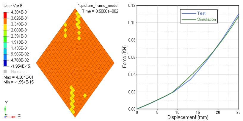
Рисунок 367: Моделирование рамки картины и напряжение сдвига как функция угла анизотропии

Можно провести циклические испытания рамки картины с нагрузкой и разгрузкой для извлечения кривых нагрузки и разгрузки при сдвиге. Кривые можно непосредственно использовать в качестве входных данных в материале LAW58. Кривые должны быть указаны как для отрицательных, так и для положительных значений угла анизотропии в градусах.

Двуосный тест определяет жесткость LAW58 в направлениях утка и обмотки.

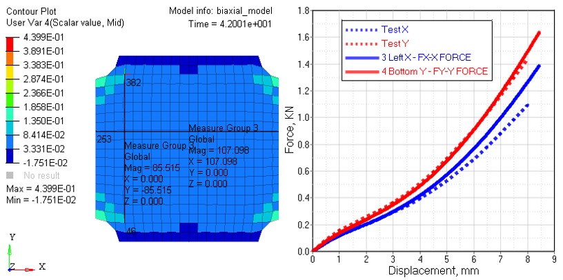
Рисунок 368: Двуосное моделирование и кривые смещения сил в направлениях основы и утка

Кривые смещения сил для направления основы и утка можно пересчитать в кривые напряжения и деформации с использованием размера и толщины образца. Из-за эффектов угловых границ может потребоваться небольшое масштабирование или другая настройка входных кривых.

Прежде чем тканые волокна основы и утка станут прямыми, данные одноосного испытания могут использоваться для проверки начальной жесткости ткани для LAW58. Во время этой фазы ткань обычно мягче. Параметры выпрямления деформации S₁ и S₂ определяют, когда деформация, когда волокна прямые. Flex₁ и Flex₂ являются коэффициентами масштабирования, которые уменьшают жесткость кривых основы и утка, пока волокна не прямые. Во многих случаях фаза очень короткая и ее можно игнорировать, определив S₁=S₂=1e-03.

Параметры Flex₁ и Flex₂ также используются для уменьшения жесткости ткани в направлении основы и утка при сжатии. По умолчанию Flex₁=Flex₂=Flex=0,01.

Данные одноосного испытания для ориентации волокон 0, 90 и 45 градусов можно использовать для двойной проверки данных материала LAW58 ткани подушки безопасности, которые были проверены с помощью испытания рамки изображения и двухосного испытания.

Стринги подушки безопасности обычно нагружаются при одноосном растяжении. Испытания на одноосное растяжение должны быть завершены и проверены для этих материалов. Проверка образцов, ориентированных под углом 45 градусов, также важна для этих материалов.

Материалы LAW58 могут включать эффект гистерезиса при циклической нагрузке. Кривые напряжения-деформации для нагрузки и разгрузки должны быть извлечены из циклического испытания на двухосное растяжение.

Общие материалы LAW58 в кг, мм, мс с опцией нагрузки и разгрузки с опцией нагрузки и разгрузки.

#---1----|----2----|----3----|----4----|----5----|----6----|----7----|----8----|----9----|---10----|
/MAT/LAW58/2
Laduga test fabric law58
#              RHO_I              RHO_O
                8E-7                  0
#                E1                  B1                   E2                  B2                FLEX
               0.380                  0                 0.380                  0                 1.0
#                G0                  GT                 AlphaT0              Gsh               sens_ID
               0.0035            0.0055                  7.175                                    1
#                Df                  Ds                  Gfrot                               ZEROSTRESS
                  0                   0                     0                                     1
#       N1        N2                  S1                   S2
           1      1                   0                     0
#      Dir 1
        500.          1.00
#      Dir 2

        501.           1.00
#      Dir12
        502.           1.00
#   FCT_ID4   FCT_ID5           Fscale4               Fscale5        FCT_ID6                   Fscale6
        600       600                 1                     1            502                            1

/FUNCT/500
кривая напряжение-деформация напр. 1
# X Y
0.0000000000e+000 0
1.0000000000e-002 2.9343543750e-003
2.0000000000e-002 5.2630337500e-003
3.0000000000e-002 6.9235412500e-003
4.0000000000e-002 8.4176677083e-003
5.0000000000e-002 1.0120216458e-002
6.0000000000e-002 1.2102790000e-002
7.0000000000e-002 1.4219608542e-002
8.0000000000e-002 1.6595997708e-002
9.0000000000e-002 1.9202795833e-002
1.0000000000e-001 2.2040856250e-002
1.1000000000e-001 2.5270391667e-002
1.2000000000e-001 2.8711702083e-002
1.3000000000e-001 3.2558656250e-002
1.4000000000e-001 3.6676625000e-002
1.5000000000e-001 4.1031145833e-002
1.6000000000e-001 4.5697987500e-002
/FUNCT/600
кривая напряжения-деформации при разгрузке 1, 2
#                 X                 Y
0.0000000000e+000 0.0000000000e+000
2.0000000000e-002 5.0000000000e-004
4.0000000000e-002 1.0000000000e-003
6.0000000000e-002 2.0000000000e-003
8.0000000000e-002 5.0000000000e-003
1.0000000000e-001 1.0000000000e-002
1.2000000000e-001 3.0000000000e-002
1.4000000000e-001 7.0000000000e-002
#---1----|----2----|----3----|----4----|----5----|----6----|----7----|----8----|----9----|---10----|
/FUNCT/501

кривая напряжение-деформация напр. 2

# X Y 0.0000000000e+000 0 1.0000000000e-002 3.7475658333e-003 2.0000000000e-002 6.4746864583e-003 3.0000000000e-002 8.6433156250e-003 4.0000000000e-002 1.0769805833e-002 5.0000000000e-002 1.2923027083e-002 6.0000000000e-002 1.5325416250e-002 7.0000000000e-002 1.8090380208e-002 8.0000000000e-002 2.1231860417e-002 9.0000000000e-002 2.4870956250e-002 1.0000000000e-001 2.8884937500e-002 1.1000000000e-001 3.3246235417e-002 1.2000000000e-001 3.8027027083e-002 1.3000000000e-001 4.3127925000e-002 1.4000000000e-001 4.8519200000e-002 1.5000000000e-001 5.4217816667e-002 1.6000000000e-001 6.0077625000e-002 #—1—-|----2----|—-3—-|----4----|—-5—-|----6----|—-7—-|----8----|—-9—-|---10----| /FUNCT/502 кривая напряжение-деформация напр. 12 # X Y -1.8803485061e+001 -1.5770466522e-003 -1.8097254117e+001 -1.5114614261e-003 -1.7387852291e+001 -1.4413505922e-003 -1.6675208927e+001 -1.3674267252e-003 -1.5959251230e+001 -1.2915012899e-003 -1.5239904181e+001 -1.2138769816e-003 -1.4517090425e+001 -1.1332172636e-003 -1.3790730171e+001 -1.0497187778e-003 -1.3060741077e+001 -9.6747019039e-004 -1.2327038129e+001 -8.8635494868e-004 -1.1589533515e+001 -8.0307143684e-004 -1.0848136486e+001 -7.1778894110e-004 -1.0102753220e+001 -6.4282044814e-004 -9.3532866620e+000 -5.8468504129e-004 -8.5996363643e+000 -5.2563223081e-004 -7.8416983143e+000 -4.6541585980e-004 -7.0793647491e+000 -4.0614312591e-004 -6.3125239587e+000 -3.6168074948e-004 -5.5410600764e+000 -3.1690734331e-004 -4.7648528535e+000 -2.7145205177e-004 -3.9837774194e+000 -2.2537031107e-004 -3.1977040240e+000 -1.8050370403e-004 -2.4064977614e+000 -1.3620800862e-004 -1.6100182740e+000 -9.1442121733e-005 -8.0811943303e-001 -4.6243379765e-005

0 0

8.0811943303e-001 4.6243379765e-005 1.6100182740e+000 9.1442121733e-005 2.4064977614e+000 1.3620800862e-004 3.1977040240e+000 1.8050370403e-004 3.9837774194e+000 2.2537031107e-004 4.7648528535e+000 2.7145205177e-004 5.5410600764e+000 3.1690734331e-004 6.3125239587e+000 3.6168074948e-004 7.0793647491e+000 4.0614312591e-004 7.8416983143e+000 4.6541585980e-004 8.5996363643e+000 5.2563223081e-004 9.3532866620e+000 5.8468504129e-004 1.0102753220e+001 6.4282044814e-004 1.0848136486e+001 7.1778894110e-004 1.1589533515e+001 8.0307143684e-004 1.2327038129e+001 8.8635494868e-004 1.3060741077e+001 9.6747019039e-004 1.3790730171e+001 1.0497187778e-003 1.4517090425e+001 1.1332172636e-003 1.5239904181e+001 1.2138769816e-003 1.5959251230e+001 1.2915012899e-003 1.6675208927e+001 1.3674267252e-003 1.7387852291e+001 1.4413505922e-003 1.8097254117e+001 1.5114614261e-003 1.8803485061e+001 1.5770466522e-003 #—1—-|----2----|—-3—-|----4----|—-5—-|----6----|—-7—-|----8----|—-9—-|---10----|

Входные кривые в LAW58 должны монотонно увеличиваться. Кривые напряжения-деформации в направлении основы и утка должны иметь ровно 2 точки пересечения: при деформации 0 и некоторой положительной деформации. Кривая напряжения сдвига в зависимости от угла анизотропии должна иметь 3 точки пересечения: при угле 0, одном положительном и одном отрицательном угле. Все кривые нагрузки и разгрузки должны быть указаны.

Необходимо задать параметр материала ZEROSTRESS=1 и использовать датчик в определении материала LAW58 для активации исходной геометрии подушки безопасности. Это должен быть тот же датчик, который используется для начала первой инъекции в /MONVOL/FVMBAG1.

Карты свойств для ткани подушки безопасности

Свойство /PROP/TYPE16 (SH_FABR) следует использовать с LAW58.

Общая карта /PROP для использования с LAW58, кг, мм, мс для подушки безопасности с элементами tria.

#---1----|----2----|----3----|----4----|----5----|----6----|----7----|----8----|----9----|---10----|
/PROP/TYPE16/1
Оболочка
#   Ishell    Ismstr     Ish3n
         4         4         2
#                 hm                  hf                  hr                 dm                  dn
                   0                   0                   0                  0                   0
#        N   Istrain               Thick              Ashear             Ithick      Iplas
         1         0                 0.3                   0                  0          0
#                 Vx                  Vy                  Vz      Isk      Ipos
                   1                   0                   0        0         0
#                Phi               Alpha               Thick                  Z        Mat
                   0                   0                 0.3                  0          1
#---1----|----2----|----3----|----4----|----5----|----6----|----7----|----8----|----9----|---10----|

Для ткани нет жесткости на изгиб. Поэтому для свойства ткани подушки безопасности следует использовать формулировку мембраны N=1. Подушки безопасности должны быть сеткой с элементами tria со следующими параметрами свойств: \(I_{shell} =4 \) и \(I_{sh3n} =2\)

Четыре оболочки узлов можно использовать с версии 2021.2. В этом случае следует использовать \(I_{shell} =12\), \(I_{smstr} =4\).

В свойстве /PROP/TYPE16 (SH_FABR) материал ткани определяется для каждого слоя. Это должен быть точно такой же материал, который используется в определении карты /PART.

Начальные направления материала определяются указанием глобальных \(V_{x}, V_{y},\) и \(V_{s}\) векторов. Векторы проецируются на каждый элемент опорной геометрии подушки безопасности и затем поворачиваются на угол Phi. Это дает первое направление материала. Второе направление материала по умолчанию перпендикулярно первому направлению или может быть указано с помощью ввода Alpha.

Примечание: Параметры по умолчанию песочных часов и коэффициенты демпфирования \(h_{m}, h_{f}, h_{r}, d_{m},\) и \(d_{n}\) работают хорошо, когда качество складывания подушки безопасности хорошее.

Моделирование подушек безопасности методом конечного объема

В PRADIOS стандартным методом расчета подушек безопасности является метод конечного объема (FVM).

FVM моделирует поток газа внутри подушки безопасности, включая взаимодействие с внутренними компонентами подушки безопасности, которые могут включать внутренние стенки, перегородки и т. д. Карты подушек безопасности /MONVOL/FVMBAG1 и /MONVOL/FVMBAG2 используются для настройки подушки безопасности FVM. Подушки безопасности с равномерным давлением можно использовать для отладки, чтобы проверить развертывание, контакты и глобальную согласованность газодинамических параметров. /MONVOL/AIRBAG1 можно использовать для активации подушки безопасности с равномерным давлением для отладки.

Универсальная карта /FVMBAG1:

/MONVOL/FVMBAG1/46
FVMBAG1
#surf_IDex                         Hconv
  666000001                            0
#              AscaleT           AscaleP           AscaleS           AscaleA              AscaleD
                     0                 0                 0                 0                    0
#    mat_ID                                           Pext             T0        Iequi       Ittf
  666400002                                           1E-4               296         1          3
# Njet
1
# inject_ID   sens_IDsurf_IDinj
  666400002 666000500 666200211
# fct_IDvel                    Fscalevel
 666000200                             1
#    Nvent  Nporsurf
         1         2
# surf_IDv     Iform               Avent             Bvent                             vent_title
 666000015         1                   0                 0
#             Tstart               Tstop             dPdef            dtPdef              IdtPdef
                   0                1E30                 0                 0                    0
#  fct_IDt   fct_IDP             fct_IDA           Fscalet           FscaleP              FscaleA
         0         0                   0                 1                 1                    1
#  fct_IDt'  fct_IDP'            fct_IDA'          Fscalet'          FscaleP'             FscaleA'
         0         0                   0                 1                 1                    1
#surf_IDps   Iformps           Iblockage                                            surface_title
 666000004         2                   0
#             Tstart               Tstop             dPdef            dtPdef              IdtPdef
                   0                   0                 0                 0                    0
#  fct_IDv                       Fscalev
 666000004                             1
#surf_IDps   Iformps           Iblockage                                            surface_title
 666000003         2                   0
#             Tstart               Tstop             dPdef            dtPdef              IdtPdef
                   0                   0                 0                 0                    0
#  fct_IDv                       Fscalev
 666000003                             1
# frame_ID     kmesh             Tswitch
         0         4                  20
#                 L1                  L2                L3
                   0                   0                 0
#      Nb1       Nb2       Nb3 grbric_ID    surf_IDin Iref
         0         0        0          0        0        0
#   Igmerg                        Cgmerg            Cnmerg             Ptole
         0                         1e-04              1E-4                 0
#                 qa                  qb              Hmin        delta_Tsca           delta_Tmin
                   0                   0                 0                 0                    0
#   Ilvout    Nlayer     Nfacmax  Nppmax            Ifvani
         1         0           0       0                 0

Общий /FVMBAG2 card:

/MONVOL/FVMBAG2/46
FVMBAG2
# surf_IDex surf_IDin              Hconv
  666000001                            0
#    mat_ID                                           Pext                T0                 Ittf
  666400002                                          1e-04               296                    3
#      Njet
          1
# inject_ID sens_IDsurf_IDinj
  666400002 666000500 666200211
#     Nvent  Nporsurf
          1         2
#  surf_IDv     Iform              Avent             Bvent                             vent_title
  666000015         1                  0                 0
#              Tstart              Tstop             dPdef            dtPdef              IdtPdef
                    0               1E30                 0                 0                    0
#   fct_IDt   fct_IDP            fct_IDA           Fscalet           FscaleP              FscaleA
          0         0                  0                 1                 1                    1
#   fct_IDt'  fct_IDP'           fct_IDA'          Fscalet'          FscaleP'             FscaleA'
          0         0                  0                 1                 1                    1
# surf_IDps   Iformps          Iblockage                                            surface_title
  666000004         2                  0
#              Tstart              Tstop             dPdef            dtPdef              IdtPdef
                    0                  0                 0                 0                    0
#   fct_IDv                      Fscalev
  666000004                            1
# surf_IDps   Iformps          Iblockage                                            surface_title
  666000003         2                  0
#              Tstart              Tstop             dPdef            dtPdef              IdtPdef
                    0                  0                 0                 0                    0
#  fct_IDv                       Fscalev
 666000003                             1
#               Cmerg            Tswitch           Iswitch           Pswitch
                1e-04               20.0                 0               0.0
#                 CFL             DT_min
                  0.0                0.0

Карта /MONVOL/FVMBAG2 доступна с 2021.1. Это точная копия карты /MONVOL/FVMBAG1. Устаревшие и неиспользуемые входные данные удалены из /MONVOL/FVMBAG2. Это делает ее простой и легкой в ​​использовании. Некоторые различия в результатах между картой /MONVOL/FVMBAG1 и /MONVOL/FVMBAG1 могут возникнуть, когда скорость впрыска в /MONVOL//FVMBAG1 установлена ​​отличной от 300 м/с. Это значение жестко закодировано в карте /MONVOL/FVMBAG2.

Внешняя поверхность закрытой подушки безопасности должна быть определена с помощью /SURF/PART и ссылаться на набор компонентов оболочки с нормалями, направленными наружу.

Параметры масштабирования Ascale_T, Ascale_P, Ascale_S, Ascale_A и Ascale_D не используются.

Атмосферные значения определяются для исходного материала воздуха, исходной температуры и исходного давления.

Параметр \(I_{ttf}\) должен быть установлен на 3. В этом случае вентиляционные отверстия активируются при TTF первого инжектора, указанном в датчике, указанном в /MONVOL/FVMBAG1, и все зависящие от времени параметры и кривые, контролирующие отверстия вентиляционных отверстий и пористость, будут смещены на время активации датчика первого инжектора.

Количество инжекторов указывается флагом \(N_{jet}\). Элементы, используемые как поверхность впрыска, должны быть помещены в отдельный компонент PART, который принадлежит либо внешней, либо внутренней поверхности подушки безопасности.

Разные инжекторы не могут использовать одни и те же элементы для поверхностей инжектора.

Время до срабатывания (TTF) для начала впрыска газа должно быть определено в /SENSOR. Глобальное определение параметра /PARAMETER может использоваться для параметризации ввода TTF и других параметров подушки безопасности.

Функция для скорости впрыска должна быть установлена ​​на постоянное значение, приблизительно равное скорости звука впрыскиваемого газа. Эта функция не оказывает существенного влияния на результаты моделирования.

Следует использовать опцию \(I_{equil}\) =1. Опция обеспечивает упрощенный цикл FVM перед TTF.

Функция для скорости впрыска должна быть установлена ​​на постоянном значении, приблизительно равном скорости звука впрыскиваемого газа. Эта функция не оказывает существенного влияния на результаты моделирования.

Внутренние поверхности (внутренние стенки, перегородки и т. д.) должны быть определены как совокупность компонентов и указаны в поле :mat h:surf_ID_{in}.

Настоятельно рекомендуется закрыть все важные межкамерные отверстия с помощью отдельных пустотных компонентов со всеми узлами, прикрепленными к тканевому компоненту. Это следует сделать до складывания подушки безопасности, чтобы избежать пересечений с другими компонентами подушки безопасности. При добавлении этих пустотных элементов конечные объемы, которые принадлежат разным камерам подушки безопасности во время моделирования развертывания, не будут объединены во время моделирования. Это также позволяет контролировать выходной и управляющий массовый поток между разными камерами подушки безопасности с помощью /TH/SURF.

Примечание: Внешние и внутренние компоненты подушки безопасности, межкамерные пустоты и пустотные компоненты, представляющие вентиляцию, не должны иметь геометрических пересечений. Создание сетки конечного объема невозможно при наличии любого пересечения.

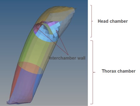
Рисунок 369: Простая рукавная подушка безопасности с 2 камерами

Начальная сетка конечного объема создается автоматически, когда используется опция /MONVOL/FVMBAG1 Kmesh=14 и не задана вручную созданная начальная тетрасетка конечного объема, как описано в следующем разделе. Затем подушка безопасности проверяется, чтобы убедиться, что на внешних и внутренних поверхностях подушки безопасности нет пересечений. Если пересечений нет, создается сетка конечного объема. Если сетка конечного объема не может быть создана из-за пересечений в компонентах подушки безопасности, выводится

сообщение об ошибке с

возможными номерами узлов/элементов и позициями, которые вызывают проблему с созданием сетки конечного объема. Когда это происходит, HyperMesh можно использовать для проверки и устранения проблем с сеткой подушки безопасности. Используйте опцию check 2Dmesh на панели tetramesh с настройками по умолчанию, чтобы проверить, приемлемы ли внешние и внутренние компоненты подушки безопасности для генерации тетрасетки.

Тетрасетка, созданная PRADIOS, выводится как включаемый файл PRADIOS MONVOL.

В случае использования четырех узловых оболочек (это возможно с версии 2021.2) PRADIOS выполняет так называемое «умное разделение» для разделения четырех узловых оболочек на трехузловые оболочки без добавления пересечений. После разделения PRADIOS создает тетрасетку как обычно.

Примечание: сетка «smart split» используется только для создания сетки тетра. В этом случае вся симуляция выполняется с использованием исходной сетки оболочки из четырех узлов и оболочки триа.

HyperMesh также можно использовать для ручного создания исходной сетки конечного объема в виде тетраэлементов.

В этом случае все внешние и внутренние компоненты подушки безопасности должны быть определены при создании сетки. Параметр

«Фиксированные триасы/квады в тетрасетке» следует использовать, чтобы убедиться, что исходная поверхностная

сетка не изменена. Использование параметра

tetramesh option «check 2Dmesh» с настройкой по умолчанию позволяет проверить, приемлемы ли внешние и внутренние компоненты подушки безопасности для создания тетрасетки.

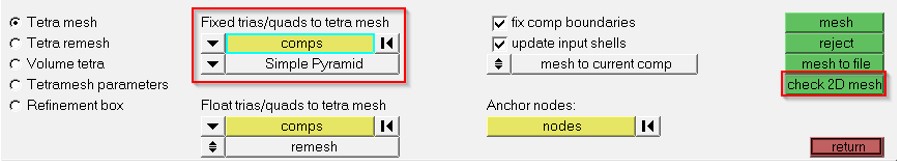
Рисунок 370:

Элементы исходной сетки конечного объема /TETRA4 следует поместить в отдельный /PART и назначить материал /MAT/VOID и свойство /PROP/VOID. Сетка должна полностью заполнять объем подушки безопасности.

Пример определения тетракомпонента исходной сетки конечного объема внутри подушки безопасности:

#---1----|----2----|----3----|----4----|----5----|----6----|----7----|----8----|----9----|---10----|
/PART/8
TETRA4
         8          8           0
/MAT/VOID/8
tetra
/PROP/VOID/8
tetra
#---1----|----2----|----3----|----4----|----5----|----6----|----7----|----8----|----9----|---10----|

Чтобы убедиться, что сетка тетра заполняет весь внутренний объем подушки безопасности, проверьте в выходном файле Starter, что НАЧАЛЬНЫЙ ОБЪЕМ КОНТРОЛИРУЕМОГО ОБЪЕМА = СУММА ОБЪЕМА КОНЕЧНЫХ ОБЪЕМОВ, указанных в том же файле. Также проверьте, что КОЛИЧЕСТВО КОНЕЧНЫХ ОБЪЕМОВ (1568 в данном случае) совпадает с количеством тетра, созданных в HyperMesh.

 НАЧАЛЬНЫЙ ОБЪЕМ КОНТРОЛИРУЕМОГО ОБЪЕМА. . .= 299199.9998912

 НОМЕР ОБЪЕМА 1
 КОЛИЧЕСТВО ПОВЕРХНОСТНЫХ МНОГОУГОЛЬНИКОВ. . . . . . .= 1200
 КОЛИЧЕСТВО ПОВЕРХНОСТНЫХ ТРЕУГОЛЬНИКОВ. . . . . .= 1200
 КОЛИЧЕСТВО КОММУНИКАЦИОННЫХ МНОГОУГОЛЬНИКОВ. . . .= 2536
 КОЛИЧЕСТВО КОММУНИКАЦИОННЫХ ТРЕУГОЛЬНИКОВ. . . . . .= 2536
 КОЛИЧЕСТВО КОНЕЧНЫХ ОБЪЕМОВ. . . . . . .= *1568*
 МИНИМАЛЬНЫЙ ОБЪЕМ КОНЕЧНОГО ОБЪЕМА. . . . . . . .= 66.66666700000 (ИДЕНТИФИКАТОР КОНЕЧНОГО ОБЪЕМА 292)
 НАЧАЛЬНЫЙ ОБЪЕМ ОБЪЕДИНЕНИЯ. . . . . . . . .= 19.08163264612
 СУММА ОБЪЕМА КОНЕЧНЫХ ОБЪЕМОВ. . . . . .= 299199.9998912
 СУММА ПЛОЩАДЬ ПОВЕРХНОСТИ ТРЕУГОЛЬНИКОВ. . . . . . .= 230031.1439046
СУММА МАССЫ КОНЕЧНЫХ ОБЪЕМОВ. . . . . . .= 3.9428379122204E-04

Если тетрасетка, созданная в HyperMesh, не полностью заполняет объем подушки безопасности, то PRADIOS попытается заполнить дополнительный объем. Когда это происходит, в выходном файле Starter появляется следующее предупреждающее сообщение.

Качество сетки тетраэдра не важно, поскольку конечные объемы, основанные на сетке тетраэдра, будут объединены в соответствии со стратегией, предоставленной параметрами слияния. \(I_{gmerg,}C_{gmerg,}\), и \(C_{nmerg,}\) можно ввести в /MONVOL/FVMBAG1. Однако рекомендуется деактивировать процесс слияния во время инициализации стартера, установив \(C_{gmerg,} = C_{nmerg,}\) 1e-04 и использовать расширенный алгоритм слияния в движке, где те же параметры можно определить в /FVMBAG/MODIF или /DT/FVMBAG/Iflag.

Начиная с версии 2019.1 параметры слияния и параметры временного шага можно вводить непосредственно в карты /MONVOL/FVMBAG1 и /MONOL/FVMBAG2.

Если /MONVOL/FVMBAG1 \(I_{f vani}\) =1, то файл анимации *A000 показывает начальные Конечные Объемы.

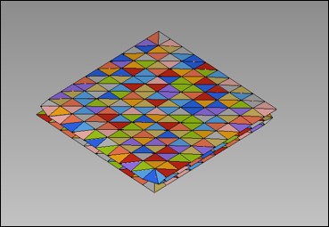
Рисунок 371: Представление начальных конечных объемов в * ``*A000`` *Файл

Количество элементов тетра зависит от сложности и типа подушки безопасности. Например, боковая подушка безопасности может содержать около 30 000–50 000 тетра, а шторная подушка безопасности — 250 000–500 000 тетра.

Опция автоматического построения сетки объема /MONVOL/FVMBAG1 Kmesh=1, не следует использовать. Рекомендуется либо использовать Kmesh=14 (сетка тетра HyperMesh), либо вручную создать тетрасетку в HyperMesh.

Вентиляционные отверстия

Каждое вентиляционное отверстие должно быть представлено как отдельный компонент в том же положении, что и в геометрии САПР.

Вентиляционное отверстие моделируется с использованием материала и свойства пустоты. Все узлы компонентов пустоты должны быть соединены с компонентом ткани. Плотность, модуль Юнга и толщина должны быть определены для компонентов пустоты с использованием тех же значений, что и для материала ткани подушки безопасности. Эти значения важны для контакта, определенного между компонентами пустоты, что помогает поддерживать внутренние объемы подушки безопасности.

Материал и свойство для компонента пустоты:

#---1----|----2----|----3----|----4----|----5----|----6----|----7----|----8----|----9----|---10----|
/MAT/VOID/2
Материальная пустота
#                RHO                   E
                8E-7                0.38
#---1----|----2----|----3----|----4----|----5----|----6----|----7----|----8----|----9----|---10----|
Недвижимость недействительна
/PROP/VOID/2
Недвижимость недействительна
#              Толстый
                 0.3
#---1----|----2----|----3----|----4----|----5----|----6----|----7----|----8----|----9----|---10----|

Если элемент упоминается в двух разных определениях вентиляционных отверстий или пористой поверхности, то элемент будет использоваться в последнем определении и удален из первого определения (это ограничение было снято в версии 2017.2.3).

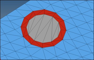
Рисунок 372: Синий — ткань подушки безопасности; Серый — вентиляционное отверстие; Красный — компонент, отделяющий вентиляционное отверстие от остальной части подушки безопасности

Определение изэнтальпического вентиляционного отверстия и пороговая функция для активации вентиляционного отверстия (кг, мм, мс)

/MONVOL/FVMBAG1
……….
#  Sid_vent         Ivent          Avent          Bvent
  666000015             1              1              0
#                  Tstart          Tstop          dPdef          dtPdef         Idtpdef
                     1E30              0          1E-06               0               0
#   fct_IDt       fct_IDP  fct_IDA              Fscalet         FscaleP         FscaleA
          0           123        0                    0               0               0
#   fct_IDt'      fct_IDP' fct_IDA'             Fscalet'        FscaleP'        FscaleA'
          0             0        0                    0               0               0
………
/FUNCT/123
1 функция масштабирования площади вентиляционного отверстия
#                       X              Y
                       -1              0
                        0              0
                    1e-06              0
                    2e-06              1
                        1              1

Вентиляционное отверстие может быть активировано при \(T_{start}\) или при достижении избыточного давления, определенного \(\Delta P_{def}\). Чтобы использовать только \(T_{start}\), определите большое значение \(\Delta P_{def}\). Чтобы использовать только \(\Delta P_{def}\), определите большое значение \(T_{start}\). При использовании \(\Delta P_{def}\) рекомендуется использовать 1e-06 ГПа (1% атмосферного давления).

Starter выводит список элементов, которые относятся к каждому вентиляционному отверстию.

ELEM: 46991 <-> SH3N : 55089506 - ВЕНТИЛЯЦИОННОЕ ОТВЕРСТИЕ: 1
ELEM: 46992 <-> SH3N : 55089507 - ВЕНТИЛЯЦИОННОЕ ОТВЕРСТИЕ: 1
ELEM: 46993 <-> SH3N : 55089508 - ВЕНТИЛЯЦИОННОЕ ОТВЕРСТИЕ: 1
ELM:  46994 <-> SH3N : 55089509 - ВЕНТИЛЯЦИОННОЕ ОТВЕРСТИЕ: 1
ELEM: 46995 <-> SH3N : 55089510 - ВЕНТИЛЯЦИОННОЕ ОТВЕРСТИЕ: 1
ELEM: 46996 <-> SH3N : 55089511 - ВЕНТИЛЯЦИОННОЕ ОТВЕРСТИЕ: 1
ELEM: 46997 <-> SH3N : 55089512 - ВЕНТИЛЯЦИОННОЕ ОТВЕРСТИЕ: 1

Dв процессе проектирования изменение диаметра вентиляционного отверстия можно упростить, создав несколько круглых компонентов для заполнения области вентиляционного отверстия. Диаметр вентиляционного отверстия можно затем легко изменить, изменяя детали, которые определяют поверхность вентиляционного отверстия. При использовании этого метода вентиляционные отверстия нельзя моделировать с использованием свойств VOID, потому что не все элементы вентиляционного отверстия прикреплены к ткани подушки безопасности. Упрощенный ортотропный LAW19 также можно использовать для представления тканевого материала круглых вентиляционных отверстий, но с уменьшенной жесткостью.

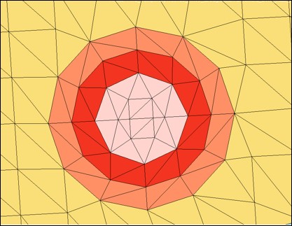
Рисунок 373: Вентиляционное отверстие с переменным диаметром

Края щелевого отверстия могут быть соединены с помощью жестких пружин /PROP/TYPE4 для обеспечения правильного складывания подушки безопасности в области около щелевого отверстия. Пружины также могут использоваться для изменения длины щелевого отверстия. Закрытые края отверстия должны быть смоделированы с помощью жестких пружин, чтобы избежать открытия.

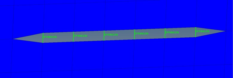
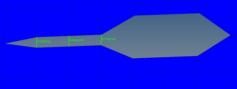
Рисунок 374: Моделирование щелевого отверстия

Пористость ткани подушки безопасности

Пористость материала подушки безопасности моделируется путем добавления карты пористости /LEAK/MAT к карте /MAT/LAW58.

Общие контакты /TYPE7 и TYPE11 между подушкой безопасности и корпусом (kg, mm, ms)

#---1----|----2----|----3----|----4----|----5----|----6----|----7----|----8----|----9----|---10----|
/MAT/LAW58/1
Закон о тестировании тканей Ладуги58
#        Init. dens.          Ref. dens.
                8E-7                   0
#                 E1                  B1                 E2                  B2                FLEX
               0.380                   0              0.380                   0                 1.0
#                 G0                  GT             AlphaT                                  Sensor
              0.0035              0.0055              7.175                                       1
#                 Df                  Ds              Gfrot                              ZeroStress
                   0                   0                  0                                       1
#       N1        N2                  S1                 S2
         1         1                   0                  0
#    Dir 1
       500.               1.00
#    Dir 2
       501.               1.00
#    Dir12
       502.               1.00
#  FCT_ID4   FCT_ID5             Fscale4            Fscale5     FCT_ID6           Fscale6
       600       600                   1                  1         502                 1
/LEAK/MAT/1
Ткань
#    Ileak             AscaleT              AscaleP
         1
#                 AC' fct_IDAC’
#                   LC                AC
             1.0e-03             1.0e-03
#---1----|----2----|----3----|----4----|----5----|----6----|----7----|----8----|----9----|---10----|

/LEAK/MAT определяет, как эффективная пористая площадь компонента, имеющего этот материал, будет изменяться в зависимости от времени или давления. Она определяется значением Ileakage.

Ileakage =1:

\[A_{eff}=\sum_{n}LC\cdot AC\cdot Area_{n}\tag{264}\]

Ileakage =2:

\[A_{eff}=\sum_{n}LC(t)\cdot AC(P)\cdot Area_{n}\tag{265}\]

Ileakage =3:

\[A_{eff}=\sum_{n}LC(t)\cdot AC(P-Pext)\cdot Area_{n}\tag{266}\]

Ileakage =4:

\[A_{eff}=\sum_{n}LC(Area_{n}/Area_{0})\cdot AC(P_{ext}/P)\cdot Area_{n}\tag{267}\]

Ileakage =5:

\[A_{eff}=\sum_{n}\frac{Area_{0}}{L^{2}}\big{[}(C_{1}\Delta P^{C_{2}}-C_{3})(L-R)^{2}+C_{3}(L\lambda_{1}-R/\sqrt{\lambda_{2}})(L\lambda_{2}-R/\sqrt\lambda_{1})\big{]}\cdot \sin a_{12} \tag{268}\]

\(\Delta P=P/P_{ext}-1\)

направления утка.

\[A_{eff}=\sum_{n}Area_{0}(X_{0}+X_{1}r_{s}+X_{2}r_{p}+X_{3}r_{s}r_{p}) \tag{269}\]

С \(r_{s}=Area_{n}/Area_{0}\) and \(r_{p}=p_{ext}/P.\)

Детали с этим материалом считаются пористыми, если ссылаться на них через идентификатор поверхности с помощью опции /MONVOL/FVMBAG1 surf_IDps.

Пример определения пористости в /MONVOL/FVMBAG1.

#---1----|----2----|----3----|----4----|----5----|----6----|----7----|----8----|----9----|---10----|
/MONVOL/FVMBAG1/1
DAB
#     Isur
         4
#             Scal_T              Scal_P              Scal_S              Scal_A              Scal_D
                   0                   0                   0                   0                   0
#   Mat_ID                            Mu                Pext                Tphi     Iequi      Ittf
         4                           0.1          0.00010135                   0         0         3
#     Njet
         1
#   Inj_ID   Isensor surf_IDinj
        10         1            100
#    Nvent       Nps
         0         1
#Sur_id_ps  Iform_ps
         4         1
#             Tstart               Tstop               dPdef              DtPdef             ldtpdef
….
#---1----|----2----|----3----|----4----|----5----|----6----|----7----|----8----|----9----|---10----|

Массовый поток через пористый материал определяется с помощью /MONVOL/FVMBAG1 \(Iform_{ps}\) и имеет следующие формулы:

\(Iform_{ps} = 1 m_{out}=A_{eff}\sqrt{2P\rho}Q^{\frac{1}{\gamma}}\sqrt{\frac{\gamma}{\gamma -1}\big{[}1-Q\frac{\gamma -1}{\gamma}\big{]}}\) (Isentropic - Wang Nefske)

\(Iform_{ps} = 2 m_{out}=A_{eff}\rho\nu(P-P_{ext})\)

Где, v скорость истечения газа (Chemkin)

\(Iform_{ps} = 3 m_{out}=A_{eff}\sqrt{2\rho(P-P_{ext})}\) (Graefe)

The \(Iform_{ps}\) =2 опция обычно используется для представления пористости ткани. Скорость выходящего газа как функция избыточного давления подушки безопасности получена из данных испытаний. .. image:: vertopal_7197fe79ded4471fa6ba70c4c62a5530/media/image126.jpg

width

3.30863in

height

1.85017in

Fiрисунок 375: Пористая ткань (желтая) отделена от проницаемого шва (красного) синим невентиляционным компонентом

Активация вентиляции и пористости ткани

Когда нет датчика для активации впрыска газа, вентиляционные отверстия и пористость становятся активными, когда \(T>T_{start,}\) или если значение давления \(P>\Delta P_{def}\) больше времени, указанного в , где все эти значения вводятся с помощью /MONVOL/FVMBAG1.

Когда хотя бы один из инжекторов активируется датчиком, то активация опций вентиляции и пористости контролируется \(I_{ttf}\).

\(T_{inj}\) - это время активации первого инжектора датчиком.

\(I_{ttf} = 0\)

	Вентиляция, Пористость
Активация	Когда:math:P>Delta P_{def} дольше, чем время \(\Delta t P_{def,}\) or \(T>T_{start}\)
ДеАктивация	\(T_{stop}\)
Функции, зависящие от времени	Нет смены

\(I_{ttf} = 3\)

	Вентиляция, Пористость
Активация	Когда \(T>T_{inj}\) и \(P> \Delta P_{def}\) longer than the time \(\Delta t P_{def,}\) or \(T>T_{inj}+T_{start}\)
ДеАктивация	\(T_{inj} + T_{stop}\)
Функции, зависящие от времени

Все остальные связанные кривые активны, когда активна соответствующая опция вентиляции, пористости или связи.

Внутренние контакты подушки безопасности

Внешние и внутренние компоненты подушки безопасности, включая межкамерные пустоты и компоненты пустот, используемые для вентиляционных отверстий, не должны иметь геометрических пересечений.

Комбинация контактов /INTER/TYPE7 и /INTER/TYPE11 должна использоваться для представления внутреннего контакта подушки безопасности.

Универсальный контакт подушки безопасности /INTER/TYPE7 (kg, mm, ms):

#---1----|----2----|----3----|----4----|----5----|----6----|----7----|----8----|----9----|---10----|
/INTER/TYPE7/666700001
Самостоятельный контакт с подушкой безопасности - 666700001
#  Slav_id   Mast_id      Istf      Ithe      Igap                Ibag      Idel     Icurv      Iadm
 666100103 666100101         4         0         0                   1         0         0         0
#          GAP_SCALE             GAP_MAX             Fpenmax
                   0                   0                   0
#              STMIN               STMAX          %MESH_SIZE               dtmin
                   1                1E30                   0                   0
#              STFAC                FRIC             GAP_MIN              Tstart               Tstop
                   1                   0                   1                   0                   0
#     I_BC                        INACTI               VIS_S               VIS_F              BUMULT
       000                             6                   0                   0                   0
#    Ifric    Ifiltr               Xfreq     Iform
         0         0                   0         2
/SURF/PART/666100101
Airbag External Surface by Part - 666100101
666000001 666000002 666000003 666000004 666000005 666000006 666000007 666000008 666000009 666000013
666000014 666000015 666000016 666000017 666000018 666000201 666000202 666000203
#---1----|----2----|----3----|----4----|----5----|----6----|----7----|----8----|----9----|---10----|

Для /INTER/TYPE7 контакта:

• Все внешние и внутренние компоненты ткани, включая межкамерные пустоты и пустотные компоненты для вентиляционных отверстий, должны быть определены в самоконтакте, где компоненты перечислены как вторичные узлы и основные поверхности

• \(I_{stf}\) =4 обеспечивает правильную жесткость контакта

• \(I_{bag}\) =1 обеспечивает закрытие вентиляционного отверстия из-за контакта

• \(St_{min}\) =1KN/mm ограничивает наименьшую жесткость контакта

• \(Gap_{min}\) =1mm обеспечивает плавное увеличение силы контакта по мере приближения вторичных узлов к основному сегменту

• Трение установлено на 0

• Inacti=6 деактивирует начальные проникновения

Начальное проникновение можно проверить с помощью средства проверки проникновений HyperCrash. Модель подушки безопасности должна быть пробита до физической толщины ткани подушки безопасности. Например, если толщина ткани подушки безопасности составляет 0,3 мм, подушка безопасности должна быть пробита до 30% от \(Gap_{min}\) = 1 значения.

Общий контакт подушки безопасности /INTER/TYPE11 (kg, mm, ms):

#---1----|----2----|----3----|----4----|----5----|----6----|----7----|----8----|----9----|---10----|
/INTER/TYPE11/666800001
Airbag Selfcontact Edge - 666800001
#  Slav_id   Mast_id     I_stf               I_gap   Multimp                Idel
 666100102 666100102         4                   0         0                   0
#              STmin               STmax           MESH_SIZE               dtmin    Iform    Sens_Id
                   1                   0                   0                   0        2          0
#              STFAC                FRIC                 GAP              Tstart               Tstop
                   1                   0                 0.9                   0                   0
#     I_BC                        INACTI               VIS_S               VIS_F              BUMULT
       000                             6                   0                   0                   0
/LINE/SURF/666100102
Airbag Line by Surface - 666100102
 666100101
#---1----|----2----|----3----|----4----|----5----|----6----|----7----|----8----|----9----|---10----|

Для /INTER/TYPE11 контакт:

• Все внешние и внутренние компоненты ткани, включая межкамерные пустоты и пустотные компоненты для вентиляционных отверстий, должны быть перечислены как на вторичной, так и на основной стороне

• \(I_{stf}\) =4 обеспечивает правильную жесткость контакта

• \(St_{min}\) =1KN/mm ограничивает наименьшую жесткость контакта

• \(Gap_{min}\) =0.9mm обеспечивает плавное увеличение силы контакта по мере приближения вторичных узлов к основному сегменту. Этот зазор контакта составляет 90% от зазора контакта /INTER/TYPE7

• Трение установлено на 0

• Inacti=6 деактивирует начальные проникновения

Начальное проникновение можно проверить с помощью средства проверки проникновений HyperCrash. Модель подушки безопасности должна быть пройдена до 90% от значения \(Gap_{min}\), что приведет к максимальному проникновению в 10% от значения \(Gap_{min}\).

Предполагая, что в модели нет начальных пересечений, определение контакта TYPE7 и TYPE11 предотвращает пересечения узлов с поверхностью и краем с краем во время моделирования подушки безопасности. Если начальные пересечения существуют в модели, модель может быть нестабильной, поскольку узлы могут застрять на неправильной стороне основной поверхности. Кроме того, сетка конечного объема не может быть создана, когда компоненты подушки безопасности имеют пересечения. Поэтому важно удалить все начальные пересечения.

При использовании опции /DT/INTER/DEL в файле Engine вторичные узлы подушек безопасности могут быть удалены из внутренних контактов, что приведет к локальным пересечениям ткани подушек безопасности и снижению точности симуляции подушек безопасности. При использовании этой опции определите локальное dtmin=1e-5ms в определении внутренних контактов /INTER/TYPE7 и /INTER/TYPE11, которое переопределит глобальное значение /DT/INTER/DEL dtmin.

Примечание: Шаг модели по времени не должен ограничиваться шагом контактной кинематики по времени.

Корпус подушки безопасности

Корпус подушки безопасности должен отображать все детали, доступные в данных САПР.

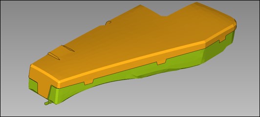
width

4.43372in

height

2.00851in

Рисунок 376: Корпус подушки безопасности

Когда подушка безопасности будет включена в полную симуляцию транспортного средства, размер и качество сетки должны быть аналогичны полному транспортному средству. Законы материалов LAW2 и LAW36 можно использовать для моделирования упругопластических материалов. Материалы с разрушением следует использовать для воспроизведения открытия крышки подушки безопасности.

Твердые пенопластовые компоненты следует моделировать с использованием LAW38 или LAW70, тогда как гиперупругие компоненты моделируются с использованием LAW42.

Свойства элемента для оболочки /PROP/TYPE1 должны использовать \(I_{shell}\) =24, чтобы избежать эффекта песочных часов. Для твердых пенопластовых или гиперупругих компонентов используйте /PROP/TYPE14 с \(I_{solid}\) =24 и \(I_{smstr}\) =10.

Контакт между подушкой безопасности и окружающей средой

Контакт между подушкой безопасности и окружающей средой следует разделить на определенные контакты:

• Подушка безопасности к нагнетателю

• Подушка безопасности к корпусу

• Подушка безопасности к манекену

• Подушка безопасности к конструкции сиденья

Общие контакты /TYPE7 и /TYPE11 между подушкой безопасности и корпусом (kg, mm, ms)

#---1----|----2----|----3----|----4----|----5----|----6----|----7----|----8----|----9----|---10----|
/INTER/TYPE7/666710001
Подушка безопасности против корпуса
#  Slav_id   Mast_id      Istf      Ithe     Igap                Ibag      Idel     Icurv      Iadm
 666100103 666200201         4         0        0                   1         2         0         0
#         Fscale_GAP             GAP_MAX            Fpenmax
                   0                   0                  0
#              STMIN               STMAX         %MESH_SIZE               dtmin
                   1                1E30                  0                   0
#              STFAC                FRIC            GAP_MIN              Tstart               Tstop
                   1                  .1                  1                   0                   0
#     I_BC                        INACTI              VIS_S               VIS_F              BUMULT
       000                             6                  0                   0                   0
#    Ifric    Ifiltr               Xfreq     Iform
         0         0                   0         2
#---1----|----2----|----3----|----4----|----5----|----6----|----7----|----8----|----9----|---10----|
/INTER/TYPE7/666710002
Подушка безопасности против корпуса
#  Slav_id   Mast_id      Istf      Ithe     Igap                Ibag      Idel     Icurv      Iadm
 666100103 666200201         4         0        0                   1         2         0         0
#         Fscale_GAP             GAP_MAX            Fpenmax
                   0                   0                  0
#              STMIN               STMAX         %MESH_SIZE               dtmin
                   1                1E30                  0                   0
#              STFAC                FRIC            GAP_MIN              Tstart               Tstop
                   1                  .1                  1                   0                   0
#     I_BC                        INACTI              VIS_S               VIS_F              BUMULT
       000                             6                  0                   0                   0
#    Ifric    Ifiltr               Xfreq     Iform
         0         0                   0         2
#---1----|----2----|----3----|----4----|----5----|----6----|----7----|----8----|----9----|---10----|
/INTER/TYPE11/666810001
Подушка безопасности против корпуса
# Slav_id   Mast_id       I_stf             I_gap   Multimp                Idel
666100102 666200203           4                 0         0                   2
#             STmin                STmax          MESH_SIZE               dtmin    Iform    Sens_Id
                  1                    0                  0                   0        2          0
#              STFAC                FRIC            GAP_MIN              Tstart               Tstop
                   1                  .1                  1                   0                   0
#     I_BC                        INACTI              VIS_S               VIS_F              BUMULT
       000                             6                  0                   0                   0
#---1----|----2----|----3----|----4----|----5----|----6----|----7----|----8----|----9----|---10----|

Обычно следует указывать два симметричных контакта /INTER/TYPE7 и один контакт /INTER/TYPE11 край к краю. Используйте следующие настройки контактов для этих контактов.

• \(I_{stf}\) =4, для обеспечения надлежащей жесткости контакта

• \(I_{bag}\) =1, для закрытия вентиляционного отверстия

• \(I_{del}\) =2, для удаления удаленных элементов из контакта

• \(St_{min}\) =1KN/mm

• \(I_{form}\) =2

Вывод истории времени и анимации

Рекомендуется запросить группу переменных по умолчанию (DEF) для вывода истории времени /TH/MONV, которая включает:

• Глобальные газодинамические параметры: масса газа, объем подушки безопасности, площадь подушки безопасности, давление (среднее), температура (среднее) и коэффициенты теплоемкости (среднее).

• Для каждого вентиляционного отверстия: площадь вентиляционного отверстия, скорость истечения и масса истечения. (По умолчанию с 2017.2.3)

• Параметры конечного объема: количество конечных объемов (NFV) и наименьший временной шаг конечного объема (DTBAG). Для версий до 2017.2.4 параметры NFV и DTBAG не были включены в вывод по умолчанию и, таким образом, должны быть определены при использовании более старых версий.

Общая карта вывода временной истории с 5 вентиляционными отверстиями

#---1----|----2----|----3----|----4----|----5----|----6----|----7----|----8----|----9----|---10----|
/TH/MONV/666000001
Airbag MonVol  История времени  - 666
#     var1      var2      var3     var4      var5      var6      var7      var8      var9     var10
DEF       NFV        DTBAG
#     Obj1      Obj2      Obj3     Obj4      Obj5      Obj6      Obj7      Obj8      Obj9     Obj10
 666000001
#---1----|----2----|----3----|----4----|----5----|----6----|----7----|----8----|----9----|---10----|

Локальное давление должно быть измерено в модели путем создания давления /МАНОМЕТРА с использованием узла ткани подушки безопасности, где давление было измерено рядом с инжектором в ходе испытания.

Общая карта выходных данных временной истории для манометра

#---1----|----2----|----3----|----4----|----5----|----6----|----7----|----8----|----9----|---10----|
/GAUGE/1
FWD
# node_ID                                          shell_ID                DIST
 50050421
#---1----|----2----|----3----|----4----|----5----|----6----|----7----|----8----|----9----|---10----|
/TH/GAUGE/1
TH GAUGE
#     var1      var2      var3     var4      var5      var6      var7      var8      var9     var10
DEF
#     Obj1      Obj2      Obj3     Obj4      Obj5      Obj6      Obj7      Obj8      Obj9     Obj10
         1
#---1----|----2----|----3----|----4----|----5----|----6----|----7----|----8----|----9----|---10----|

Массовый поток через любые проницаемые внутренние поверхности подушки безопасности можно вывести с помощью карты /TH/SURF.

Общий вывод временной истории для площади и массового потока через проницаемую внутреннюю поверхность подушки безопасности

#---1----|----2----|----3----|----4----|----5----|----6----|----7----|----8----|----9----|---10----|
/TH/SURF/666000002
Airbag MonVol Time History - 666
#     var1      var2      var3     var4      var5      var6      var7      var8      var9     var10
AREA     MASSFLOW
#     Obj1      Obj2      Obj3     Obj4      Obj5      Obj6      Obj7      Obj8      Obj9     Obj10
666000001
#---1----|----2----|----3----|----4----|----5----|----6----|----7----|----8----|----9----|---10----|

Карта должна ссылаться на поверхности, определенные /SURF.

Следующие карты должны быть определены в файле Engine для анимационного вывода давления газа, плотности, температуры и скорости жидкости в узлах поверхности подушки безопасности.

/ANIM/NODA/P or /H3D/NODA/P

/ANIM/NODA/DENS or /H3D/NODA/DENS

/ANIM/NODA/TEMP or /H3D/NODA/TEMP

/ANIM/VECT/FVEL or /H3D/NODA/FVEL

Управление временным шагом и слиянием

Временной шаг и количество конечных объемов влияют на время выполнения модели имитации подушки безопасности. В этом разделе описываются доступные параметры для влияния на временной шаг и количество конечных объемов.

Временной шаг для конечных объемов основан на исходной сетке и рассчитывается как:

\[\Delta t_{fv} =\Delta T_{sca}\cdot\left(\frac{l_{c}}{v + C}\right)\tag{270}\]

Где,

\(\Delta T_{sca}\) Time step scale factor entered in /DT/FVMBAG/1, /MONVOL/ FVMBAG1, or /MONVOL/FVMBAG2

\(l_{c}\) Характерная длина, которая является минимальной длиной ребра исходной сетки тетра конечного объема

\(v\) Максимальная скорость газа

\(C\) Максимальная скорость звука

Характерная длина рассчитывается в Starter на основе исходной сетки FV и не изменяется во время моделирования. Вывод Polyhedra предназначен для метода генерации сетки Kmesh=1, который больше не рекомендуется. Информация о минимальной длине, указанная после «КОЛИЧЕСТВО ДОПОЛНИТЕЛЬНЫХ КИРПИЧЕЙ», предназначена для автоматической генерации сетки, Kmesh=14 или если элементы конечного объема создаются вручную в HyperMesh.

FVMBAG: КОНЕЧНЫЙ ОБЪЕМ МИНИМАЛЬНАЯ ДЛИНА
  ------------------------------------
  НОМЕР ОБЪЕМА 666000001
  ОБЩЕЕ КОЛИЧЕСТВО КОНЕЧНЫХ ОБЪЕМОВ. . . . . . . .= 30610
  КОЛИЧЕСТВО МНОГОГРАННИКОВ . . . . . . . . . . . . .= 0
  МИНИМАЛЬНАЯ ДЛИНА, ИСПОЛЬЗУЕМАЯ ДЛЯ ВРЕМЕННОГО ШАГА. . . . .= 0,000000000000
  МИНИМАЛЬНАЯ ДЛИНА НА ОСНОВЕ ОБЪЕМА . . . . . .= 100000000000,00
  МИНИМАЛЬНАЯ ДЛИНА НА ОСНОВЕ УЗЛОВОГО РАССТОЯНИЯ . .= 1.0000000000000E+15
  КОЛИЧЕСТВО ДОПОЛНИТЕЛЬНЫХ КИРПИЧЕЙ . . . . . . . . .= 30610
  МИНИМАЛЬНАЯ ДЛИНА НА ОСНОВЕ ОБЪЕМА . . . . . .= 0.7039415515349
  МИНИМАЛЬНАЯ ДЛИНА НА ОСНОВЕ УЗЛОВОГО РАССТОЯНИЯ . .= 0.5268862297298
  МИНИМАЛЬНАЯ ДЛИНА НА ОСНОВЕ ОБЪЕМА/ПЛОЩАДИ. . . .= 4.9347603553545E-02

Поскольку движения газа нет, начальный временной шаг представляет собой характерную длину, деленную на скорость звука воздуха при комнатной температуре. Когда начинается впрыск, скорость газа и скорость звука газа увеличиваются, а временной шаг обычно падает в течение короткой фазы после времени до срабатывания. В этой фазе временной шаг может стать меньше целевого структурного временного шага и, таким образом, контролировать временной шаг прогона. Однако через некоторое время (обычно 5-10 мс) скорость газа уменьшается, а временной шаг и становится выше структурного временного шага. Важно минимизировать продолжительность времени, когда временной шаг подушки безопасности является самым низким временным шагом в моделировании.

Характерная длина недооценивается в моделировании, поскольку она основана на минимальной длине края сложенной подушки безопасности. Таким образом, временной шаг можно увеличить, сделав \(\Delta T_{sca}\) a value greater than 1 in /DT/FVMBAG/1.

Начиная с версии 2017.2.4, временной шаг FVM выводится по умолчанию, когда в модели используется /MONVOL/FVMBAG1. Для более старых версий необходимо определить переменную DTBAG в /TH/MONV.

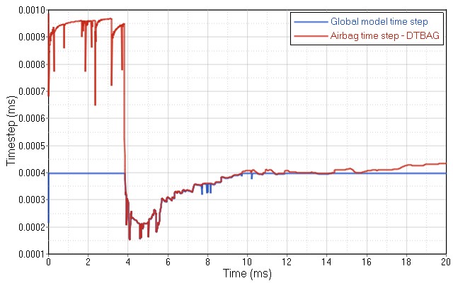
Рисунок 377: Типичная эволюция временного шага для модели с FVM Airbag (красный — глобальный временной шаг, синий — временной шаг FVM)

FVM airbag контролирует временной шаг от 3,75 мс до 7,5 мс)

Во время моделирования FV объединяются с использованием этих методов.

• Стабильное слияние: это слияние по умолчанию. FV всегда объединяется, когда его объем становится отрицательным.

• Глобальное слияние: FV объединяется, если его объем становится меньше коэффициента Cgmerg, умноженного на средний объем всех конечных объемов,

который представляет собой объем подушки безопасности, деленный на количество FV. Параметр указывается в /FVMBAG/MODIF или в /MONVOL/FVMBAG1, /MONVOL/FVMBAG2 (по состоянию на 2019.1).

• Слияние соседей: FV объединяется, если его объем становится меньше Cnmerg, умноженного на средний объем его соседних конечных объемов.

Параметр обычно указывается в карте /FVMBAG/MODIF. Этот тип слияния трудно контролировать, поэтому он не рекомендуется.

• Объединение временных шагов: FV объединяется, если его временной шаг < dtmin, определенный в картах /DT/FVMBAG/1 или /MONVOL/FVMBAG1,

/MONVOL/FVMBAG2 (по состоянию на 2019.1)

Количество конечных объемов быстро уменьшается во время моделирования. Однако важно иметь плавное уменьшение количества конечных объемов и достаточное количество (1-10% от начального числа) конечных объемов в конце моделирования. Самый простой способ контролировать слияние конечного объема — настроить параметр Cgmerg. Обычно значение должно быть между 0,01 и 0,1.

PRADIOS выводит конечное количество FV и количество объединенных FV в конце моделирования.

** КОНЕЧНЫЙ ОБЪЕМ 24 СТАТИСТИКА СЛИЯНИЯ **
   КОЛИЧЕСТВО ОСТАЛЬНЫХ КОНЕЧНЫХ ОБЪЕМОВ .....: 6999
   ГЛОБАЛЬНОЕ СЛИЯНИЕ ..............................: 22730
   СЛИЯНИЕ СОСЕДСТВА ................................: 0
   СЛИЯНИЕ СТАБИЛЬНОСТИ .................................: 885
   СЛИЯНИЕ ШАГА ВРЕМЕНИ ........................:        2

Переключение с FVM на подход равномерного давления (UP)

Параметр /MONVOL/FVMBAG1 и /MONVOL/FVMBAG2 \(T_{switch}\) можно использовать для переключения с расчета FVM на UP. Расчет UP менее затратен и, таким образом, экономит время моделирования. Переключение следует выполнять в момент стабилизации давления внутри подушки безопасности, что происходит, когда локально измеренное давление становится таким же, как и среднее давление.

Прогон стабильности

Сложенная модель подушки безопасности с правильным материалом, свойством, определением контакта и заданной геометрией отсчета не должна двигаться до активации инжектора.

Для проверки стабильности установите \(T_{delay}\) =50 мс в /SENSOR/TIME, на который ссылается /MONVOL/FVMBAG1, и запустите моделирование с конечным временем 50 мс. Модель подушки безопасности не должна показывать значительного увеличения напряжений, деформаций и нефизического движения до TTF. Если есть движение или напряжение, оно обычно вызвано контактом или какой-либо проблемой с опорной геометрией. Не используйте демпфирование /DAMP, активацию контакта или не делайте модель подушки безопасности жесткой, чтобы предотвратить движение подушки безопасности до TTF.

Корпус подушки безопасности и компоненты нагнетателя должны быть включены в прогон стабильности вместе с определением контакта между подушкой безопасности и этими компонентами.

Прогон равномерного давления

Необходимо выполнить равномерный прогон давления, чтобы убедиться, что газодинамические данные, вход инжектора, тканевые материалы и контакты дают физические результаты.

Чтобы создать равномерный тест давления:

• Заменить /MONVOL/FVMBAG1 на ключевое слово /MONVOL/AIRBAG1

• Удалить поверхность инжектора из определения инжектора

• Закомментировать входную кривую скорости инжектора

• Сохранить все вентиляционные отверстия как в подушке безопасности конечного объема

• Закомментировать информационные строки с входными данными для сетки подушки конечного объема

Преобразование /MONVOL/FVMBAG1 в /MONVOL/AIRBAG1

#---1----|----2----|----3----|----4----|----5----|----6----|----7----|----8----|----9----|---10----|
/MONVOL/AIRBAG1/1
SAB
#     Isur
         4
#           Ascale_T            Ascale_P            Ascale_S            Ascale_A            Ascale_D
                   0                   0                   0                   0                   0
#   Mat_ID                                              Pext                 T_0     Iequi      Ittf
      5000                                         1.0135E-4                 296
#     Njet
          1
#inject_ID    sens_IDsurf_IDinj
#     10001          22       19
      10001          22
##fct_IDvel                   Fscalevel
#         4                           0
#    Nvent
          0
##   Iframe
#         0
##                   l1              l2                   l3
#
##      Nb1         Nb2    Nb3grbric_ID surf_IDin       Iref
#         0           0      0       21         20          0
##   Igmerg                      Cgmerg                Cnmerg                Ptole
#         1                       1e-04                 1e-04                   0
##                   qa              qb                  Hmin
# 0
##   Ilvout      Nlayer   Nfacmax   Nppmax    ifvani
#         0           0         0        0         1
/SURF/PART/4
ВНЕШНЯЯ ПОВЕРХНОСТЬ ПОДУШКИ БЕЗОПАСНОСТИ
          1           2         4        5         6        7
#---1----|----2----|----3----|----4----|----5----|----6----|----7----|----8----|----9----|---10----|

Результаты моделирования следует визуально проверять на предмет реалистичного развертывания подушки безопасности, отсутствия застрявших или зависших узлов из-за контактных пересечений, развития временного шага, энергетического баланса и энергетической ошибки.

Параметры подушки безопасности, масса, объем, давление и температура должны быть нанесены на график и сравнены с объемом подушки безопасности и массой впрыскиваемого газа физическими характеристиками.

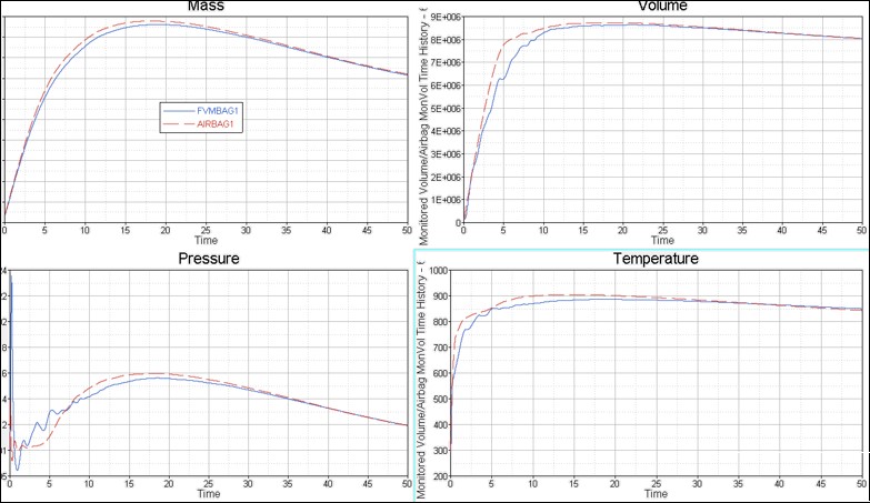
Рисунок 378: Параметры подушки безопасности для управления запуском /AIRBAG1

Для каждого вентиляционного отверстия следует нанести на график площадь вентиляционного отверстия

и выходной поток вентиляционного отверстия и сравнить их с физическим размером фактического вентиляционного отверстия в подушке безопасности.

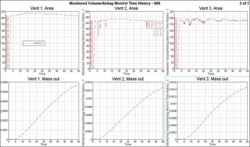
Рисунок 379:

Эти данные следует использовать в качестве базового сравнения со средними газодинамическими данными из моделирования /MONVOL/FVMBAG1.

Автономный запуск подушки безопасности FVM

Подушку безопасности FVM следует запускать автономно, чтобы проверить правильное поведение развертывания и характеристики подушки безопасности.

Параметры слияния FV и управление шагом времени можно изменить, чтобы сократить время моделирования, при этом обеспечивая реалистичные результаты.

Типичные параметры FV вводятся в файл двигателя как (также могут быть добавлены в /MONVOL/FVMBAG1, /MONVOL/FVMBAG2 cards as of 2019.1):

/DT/FVMBAG/1
1.5 1.0e-05
/FVMBAG/MODIF
666000001
1  0.010  0.001  1

Изменение коэффициента масштабирования временного шага и глобального параметра слияния может потребоваться для обеспечения правильного временного шага и количества FV в конце симуляции.

Количество конечных объемов и временной шаг FV можно отобразить в HyperGraph.

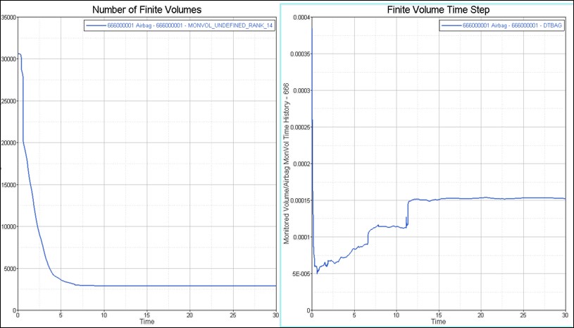
Рисунок 380:

Количество конечных объемов должно плавно уменьшаться до 2-10% от начального количества конечных элементов. Стратегия слияния также должна обеспечивать шаг времени выше минимального шага времени, требуемого в моделировании столкновений.

Слияние FV должно быть проверено в выходном файле Engine:

2 0.6688E-03 0.2863E-03 FVBAG 666000001 0.0% 2.739 0.1415E-14 0.000   -0.8103E-19
0.000
   ** ИДЕНТИФИКАТОР ОТСЛЕЖИВАЕМОГО ОБЪЕМА: ********ШАГ ВРЕМЕНИ: 0.2878E-03 КОНЕЧНЫЙ ОБЪЕМ: 21940

   ** ИДЕНТИФИКАТОР ОТСЛЕЖИВАЕМОГО ОБЪЕМА: ******** - ОБНОВЛЕНИЕ СЕТКИ КОНЕЧНОГО ОБЪЕМА **
   КОЛИЧЕСТВО КОНЕЧНЫХ ОБЪЕМОВ : 30605
   СУММА ОБЪЕМА КОНЕЧНЫХ ОБЪЕМОВ : 155386.459 (ОБЪЕМ AIRBA 155386.459 )
   СУММА ПЛОЩАДЬ ПОВЕРХНОСТИ ПОЛИГОНЫ : 227440.887 (ПЛОЩАДЬ AIRBAG 227440.887 )

   Необходимо разумное количество конечных объемов, и объединение конечных объемов не должно приводить к немедленному снижению числа до одного конечного объема.

   Конечный временной шаг объема в карте ``/DT/FVMBAG`` должен быть меньше, чем
   начальный конечный временной шаг объема, выводимый в Starter output. Параметр
   слияния *Cgmerg* в ``/FVMBAG/MODIF`` не должен быть слишком высоким, чтобы обеспечить
   гладкую историю слияния FV.

Сумма конечных объемов должна быть равна фактическому объему подушки безопасности, так как:

** ИДЕНТИФИКАТОР ОБЪЕМА: 1 - ОБНОВЛЕНИЕ СЕТИ КОНЕЧНОГО ОБЪЕМА **

КОЛИЧЕСТВО КОНЕЧНЫХ ОБЪЕМОВ: 1565 СУММА ОБЪЕМА КОНЕЧНЫХ ОБЪЕМОВ: 298121,912 (ОБЪЕМ AIRBA 298121,912) СУММА ПЛОЩАДЬ ПОВЕРХНОСТИ ПОЛИГОНОВ: 230093,158 (ОБЪЕМ AIRBAG 230093.158)

Каждый раз, когда объединяются конечные объемы, в выходных данных движка появляется это сообщение.

44  0.1320       0.2865E-02 FVBAG         1    1.0%   7.222      0.1104   0.000     0.4265E-01    0.000
** MONVOL ID        1 ОБНОВЛЕНИЕ СЕТКИ КОНЕЧНОГО ОБЪЕМА - ЦИКЛ - КОЛИЧЕСТВО КОНЕЧНЫХ ОБЪЕМОВ :    1564
** MONVOL ID        1 ОБНОВЛЕНИЕ СЕТКИ КОНЕЧНОГО ОБЪЕМА - ЦИКЛ - КОЛИЧЕСТВО КОНЕЧНЫХ ОБЪЕМОВ :    1563
** ИДЕНТИФИКАТОР КОНТРОЛИРУЕМОГО ОБЪЕМА: 1ШАГ ПО ВРЕМЕНИ: 0.4293E-02 КОНЕЧНЫЙ ОБЪЕМ: 396

Движение газа внутри подушки безопасности следует рассматривать путем контурного построения анимационного вывода температуры и скорости газа. Движение должно четко развиваться от нагнетателя в объем подушки безопасности и учитывать топологию подушки безопасности (внутренние стенки, перегородки, вентиляционные отверстия и т. д.).

Параметры газа в подушке безопасности следует сравнивать с равномерным давлением подушки безопасности. Существенные различия следует проверять и объяснять.

Рисунок 381: Сравнение выходных данных подушек безопасности для симуляций AIRBAG1 и FVMBAG1

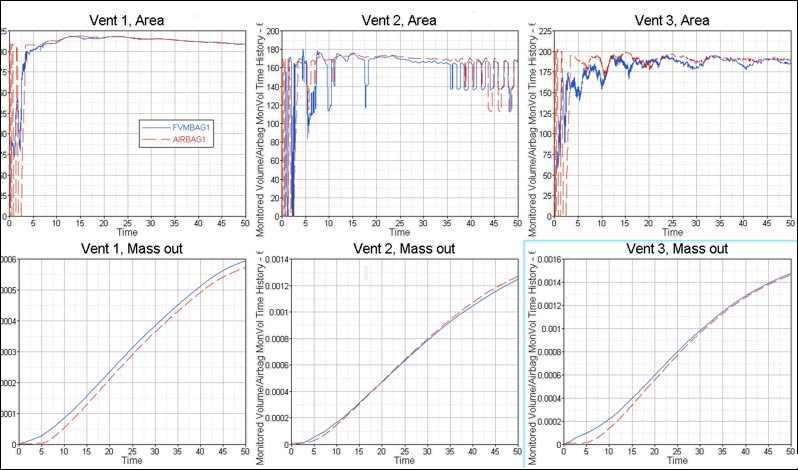
Рисунок 382: Сравнение параметров вентиляции для моделирования AIRBAG1 и FVMBAG1

Площадь вентиляции и отток вентиляции должны быть нанесены на график для каждого отверстия и контролироваться и сравниваться с равномерным ходом давления.

Устранение плохого объема

Начальная форма тетра не очень важна для расчета FVM. Объемы объединяются с соседними в соответствии с глобальными параметрами слияния Cmerge и параметром I Tscale для определения временного шага FVM.

Контрольный список

Полезный контрольный список для моделирования подушек безопасности:

• Все компоненты ткани подушки безопасности сплетены с элементами триа в соответствии с требованиями к сетке (средний размер 3-4 мм)

• Подушка безопасности не имеет пересечений

• Если подушка безопасности будет использоваться в более крупной симуляции, нумерация идентификатора сущности будет правильной на основе требований более крупной модели

• Модель подушки безопасности разделена на /SUBSET, представляющую внешние поверхности подушки безопасности, вентиляционные отверстия, внутренние поверхности, корпус и нагнетатель

• Масса и инерция модели соответствуют физической части

• Данные о материале ткани были проверены с помощью двухосных, одноосных и рамочных испытаний

• Смоделированы вентиляционные отверстия

• Смоделирована пористая ткань

• Смоделирован материал газа для каждого газового компонента

• Нагнетатель проверен с помощью моделирования испытания резервуара и сравнения кривых массового расхода и температуры с результатами испытания резервуара

• Впрыск газа начинается с TTF, определенного в /SENSOR \(T_{delay}\), а не путем смещения кривых массового расхода и температуры

• Кривая массового расхода начинается с ненулевых значений

• \(C_{p}(T)\) функция монотонно увеличивается для каждого газа

• Опорная геометрия представлена ​​либо как узловая /XREF, либо как элементная /EREF

• Тот же /SENSOR используется для активации впрыска и активации опорной геометрии в LAW58

• Указаны свойства окружающего и внутреннего воздуха

• Указана карта /FVMBAG1 или /FVMBAG2

• Определены внутренние контакты подушки безопасности, и проверка проникновения HyperCrash не показывает пересечений и максимальное проникновение 10% от зазора контакта

• Стабильность запуск выполняется для проверки движения перед TTF

• Равномерный запуск давления завершен, без закрепления узлов контакта

• Автономный запуск FVM завершен, без закрепления узлов контакта и реалистичное развертывание

• Модель запущена с требуемым шагом по времени

• Количество FV не уменьшается до одного

• Визуальное развитие потока (график контура температуры, вектор скорости жидкости) реалистично

Испытание в резервуаре

Используя данные с выходных данных испытания резервуара, можно получить температуру и массовый расход подаваемого газа, которые можно использовать в качестве входных данных для PRADIOS.

При испытании резервуара можно измерить давление в точке впрыска или в середине резервуара, эти два значения равны, поэтому изменение давления хорошо известно. Кроме того, известны количество подаваемого газа и характеристики газа в испытании.

Для температуры сложнее получить точные данные испытаний, поскольку температурные датчики часто недостаточно точны. Поэтому температура из испытания резервуара может быть неправильной.

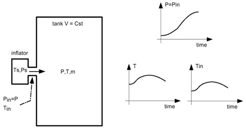
Рисунок 383: Неизвестный массовый расход

В следующих случаях учитывается, что вы можете знать или не знать температуру впрыска и температуру в баке.

В случае, если температура в инжекторе и в баке неизвестна:

• IНачальный и закачиваемый состав газа

Зная молекулярную массу (\(NW_{i}\)) каждого элемента и молярную долю (\(X_{i}\)), можно определить молярную массу газа (MW):

\[MW=\sum X_{i}\cdot MW_{i} \tag{271}\]

Средняя теплоемкость на единицу массы смеси газов определяется уравнением Амагата-Ледюка:

\[C_{p}(T)=\frac{\sum m_{i}\cdot C_{pa}}{\sum m_{i}}+\frac{\sum m_{i}\cdot C_{pb}}{\sum m_{i}}T+\frac{\sum m_{i}\cdot C_{pc}}{\sum m_{i}}T^{2}\tag{272}\]

Используя предыдущее уравнение, можно определить коэффициенты теплоемкости (\(C_{p}(T)\)) исходной и впрыскиваемой смеси.

Зная характеристики впрыскиваемого газа, исходного газа и смеси, можно найти массовый расход и температуру для инфлятора. Для проведения анализа используются следующие основные уравнения.

• Уравнение состояния идеального газа имеет вид:

\[PV=nRT,n=\frac{m}{MW}\tag{273}\]

с \(R=8.314\frac{J}{mole\cdot K}\)

• И адиабатическое уравнение:

\[H=const. \tag{274}\]

с H являясь полной энтальпией системы (нагнетатель + бак).

Из закона сохранения энергии основное уравнение энергии для теста бака можно записать как:

\[dE_{airbag}=-PdV+dH_{in}-dH_{out} \tag{275}\]

Здесь \(dH_{out}\) =0.

поэтому уравнение 275 суммируется как:

\[U_{f}-U_{0}=dH_{in}\tag{276}\]

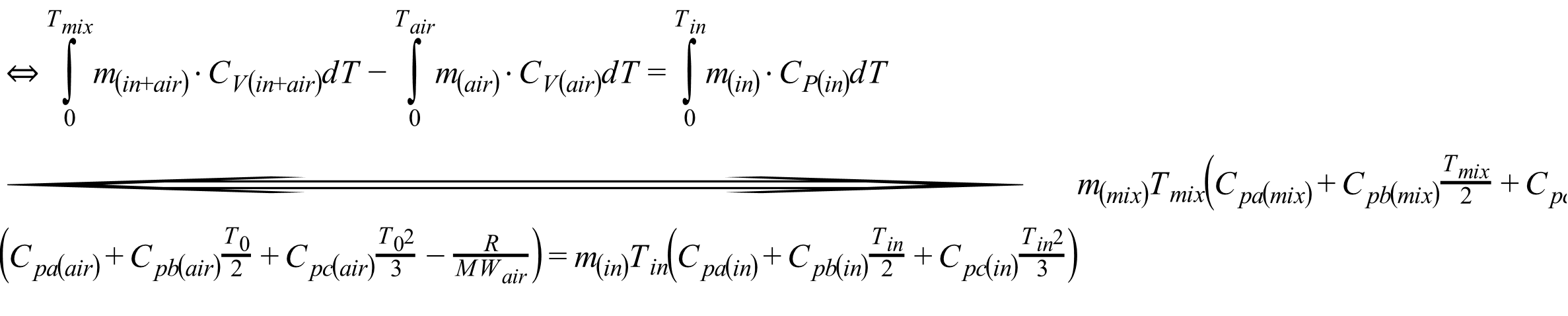
Температура инфлятора

в уравнении 276 неизвестной переменной является только \(T_{ini}\).

Другие переменные известны или могут быть определены с помощью уравнения 272 и уравнения 273:

• \(m_{(in)}m_{(air)}=MW\_{air}\frac{P_{0}V}{RT_{0}}\) и \(n_{(mix)}=\frac{m_{(in)}}{MW_{in}}+\frac{m_{(air)}}{MW_{air}}\)

• для i = a to c: \(C_{pb(in)}C_{pd(air)}C_{pb(mix)}\) рассчитываются по уравнению 272, и

• \(T_{mix}=\frac{P_{tank}V_{tank}}{n_{(mix)}R}\)

Таким образом, уравнение 276 находит температуру на инжекторе \(T_{in}\) впрыскиваемого газа путем итерации по \(T_{in}\). Сначала угадывается температура и шести итераций достаточно, чтобы сойтись к решению.

Массовый расход

Зная изменение давления в зависимости от времени в верхней части резервуара теста, можно определить массовый расход с помощью:

\[m=\frac{\partial m}{\partial P}\frac{\partial P}{\partial t}\cong\frac{\Delta M}{\Delta P}\frac{\partial P}{\partial t}\tag{277}\]

С,

\(\Delta P\) Общее изменение давления во время эксперимента

\(\Delta M\) Общая введенная масса

Уравнение 277 можно записать, если изменение массы в зависимости от изменения давления является строго растущей функцией, что и имеет место.

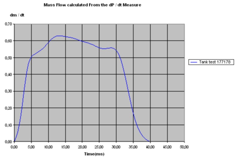
Рисунок 384: Кривая массового расхода — изменение массового расхода в зависимости от времени

Скорость газа в инфляторе

Поскольку давление быстро становится равномерным, можно записать следующее уравнение: \(P_{in}=P(t)\), зная \(T_{in}\), плотность можно выразить как функцию \(T_{in}\) и \(P(t)\):

Рекомендации по настройке подушек безопасности

Материалы подушек безопасности

Рекомендации по настройке модели материала ткани с использованием LAW19.

LAW19 опции	Рекомендуемое значение	Рекомендуемый вариант Подробности
RE	0.001 < \(R_{E}\) < 0.01	Если \(R_{E} > 0.01\) жесткость сжатия слишком высока.
ZeroStress	1	Предварительное напряжение подушки безопасности применено правильно.
sens_ID	Используйте тот же датчик, что и используется в / MONVOL карта	Предварительная деформация ткани через ссылку геометрия должна быть активируется вовремя, чтобы огонь.

Рекомендации по настройке модели тканевого материала с использованием LAW58.

Свойства подушек безопасности

Рекомендация по свойствам ткани``/PROP/TYPE9 (SH_ORTH)`` and /PROP/TYPE16 (SH_FABR).

Вариант недвижимости	Рекомендуемое значение (постоянный материал)		Рекомендуемый вариант Подробности
	LAW19	LAW58
\(I_{nh3n}\) для триаса	2	2	Это формулировка триа по умолчанию.
\(I_{smstr}\) для триаса	1	4	Рекомендации по для 3-узловых триасов передовой практике
\(I_{shell}\) для 4-х узлов. оболочек	12	12	Такая формула позволяет избежать эффекта «песочных часов».
\(I_{smstr}\) для 4- узл. оболочек	11	11	Необходимо использовать с \(I_{shell}\) =12, 4 узл. оболочка.
N	1	1	Включить разработку мембран
Thick	> 0	> 0	Толщина должна быть определена
\(I_{plas}\)	0	0	Не актуально для ткани
\(I_{thick}\)	0	0	Не актуально для ткани.
Vx, Vy, Vz	Ненулевой вектор	Ненулевой вектор	Этот вход определяет вектор который определяет сначала направление ортотропии. Если не определена глобальная ось X используется.
Idril	0	0	Не актуально для ткани

Самостоятельный контакт подушки безопасности

Если все пересечения можно удалить из подушки безопасности, то контакт поверхности с поверхностью и края и определить с помощью /INTER/TYPE19. В некоторых продвинутых случаях лучше определить два отдельных контакта, /INTER/TYPE7 для узла с поверхностью и /INTER/TYPE11 для контакта края.

Опции интерфейса	Рекомендуемые настройки для контактов TYPE7, TYPE11 и TYPE19	Комментарии
Перекрестки	Пересечения запрещены	Пересечения запрещены.
Проникновения	Проникновения < 95% разрыв	Все Проникновения > 95% разрыв нужно удалить.
\(I_{stf}\)	4	Жесткость интерфейса - это минимум основных и вторичная жесткость.
\(St_{min}\) (kN/mm)	1	Избегает слишком мягкого контакта.
\(I_{del}\)	0	Не относится к самоконтакту с подушкой безопасности.
\(I_{gap}\)	0	Используется постоянный зазор, определяемый Gapmin.
\(Gap_ {min}\)	1.0 mm	Для TYPE11, использовать \(Gap_{min}\) =0.9mm
Inacti	6	Автоматически устраняет начальные проникновения, уменьшая зазор между контактами.
Fric	0	При самоконтакте подушки безопасности трение не исп-ся.
\(I_{bag}\)	1	При контакте заблокируйте вентиляционные отверстия и пористые ткани.

Если невозможно удалить пересечения, то можно использовать /INTER/TYPE23 с этими рекомендуемыми значениями.

Опции интерфейса	**Рекомендуемые настройки для TYPE23**	Комментарии
Проникновения	Проникновения < 95% разрыва	Все проникновения > 95% разрыва необходимо удалить.
\(I_{stf}\)	4	Жесткость интерфейса - это минимум основных и вторичная жесткость.
\(I_{del}\)	0	Не актуально для подушек безопасности самоконтакт.
\(I_{gap}\)	0	Постоянный зазор используется как определение \(Gap_{min}\)
\(Gap_ {min}\)	Толщина тканевого материала	Это значение определяет как зазор между контактами и глубина контакта, тоже высокие значения будут означать что пересечённые узлы не будут выпущен из-за слишком высокого Глубина контакта.
Inacti	6	Автоматически удалять начальные проникновения за счет уменьшения Контактный зазор.
Fric	0	В подушке безопасности не используется трение самоконтакт
\(I_{bag}\)	1	Заблокируйте вентиляционные отверстия и пористые ткани при контакте.

25. Материал ткани LAW19 совместим только с /PROP/TYPE9 (SH_ORTH).

Отладка срабатывания подушки безопасности

Цель здесь — предоставить некоторые рекомендации по устранению неполадок моделирования, когда подушка безопасности не срабатывает должным образом или дает сбой из-за подушки безопасности.

Существует множество возможных причин сбоя срабатывания или сбоя моделирования из-за подушки безопасности. Здесь основное внимание уделяется наиболее распространенным проблемам.

Система единиц измерения

Проверьте плотность и модуль различных деталей и убедитесь, что они находятся в одной и той же системе единиц измерения. Например, модуль Юнга для пластиковых и металлических деталей должен быть в диапазоне:

0,01 ГПа < E < 210 ГПа

Эти значения можно проверить в HyperCrash с помощью проверки контура, расположенной в раскрывающемся меню Качество.

Неправильное определение контакта Отсутствующие контакты

Чтобы предотвратить застревание/блокировку подушки безопасности во время раскрытия, определите следующие контакты:

• Самоконтакт подушки безопасности для контакта с поверхностью и краем.

  ◦ TYPE19

  ◦ Альтернатива для некоторых моделей, требующих различных настроек для поверхностного и краевого контакта, определяет TYPE7 + TYPE11

  ◦ См. Рекомендации по настройке подушек безопасности для контакта

  • Подушка безопасности к окружающей среде (IP, рулевое колесо…)

  ◦ TYPE7: подушка безопасности является вторичной, окружающая среда является основной

  ◦ Симметричный контакт TYPE7: окружающая среда является вторичной, подушка безопасности является основной

  ◦ TYPE11: подушка безопасности является вторичной, окружающая среда является основной

  ◦ Альтернатива — определить один TYPE19 с подушкой безопасности в качестве вторичной и окружающей средой в качестве основной

  ◦ Настройка \(I_{del}\) =1 (критическая) при определении отказа

Проникновение и пересечение

Пересечения будут препятствовать правильному развертыванию подушки и должны быть устранены. Не должно быть пересечения на контакте самоудара подушки или между подушкой и окружающей средой. Пересечение можно проверить в HyperMesh или HyperCrash.

Проникновения часто встречаются при самоконтакте сложенной подушки безопасности. Идеальным случаем было бы полное отсутствие проникновения. Флаг Inacti=6 автоматически регулирует уменьшение зазора, чтобы предотвратить начальную силу контакта, вызванную проникновениями. Однако после автоматического уменьшения все еще должен быть достаточный зазор. Поэтому максимальное проникновение должно быть менее 95% от контактного зазора. Проверку проникновения можно выполнить в инструменте проверки проникновения HyperCrash или HyperMesh.

26. Материал ткани LAW58 совместим только с /PROP/TYPE16 (SH_FABR).

Датчик и опорная геометрия

Датчик, определяющий время начала впрыска подушки безопасности (TTF), /MONVOL sens_ID также должен быть указан в материале LAW19 или LAW58 sens_ID. Этот датчик позволяет решателю узнать, когда эталонная геометрия должна стать активной.

Если тот же sens_ID не используется, то может возникнуть нереалистичная деформация подушки безопасности после первых нескольких миллисекунд срабатывания и неустойчивое поведение.

Неправильный материал

Проверьте рекомендуемые значения в материалах подушек безопасности.

Неправильное свойство~~~~~~~~~~~

Поскольку геометрия подушек безопасности очень сложна, также широко используются триасы (3-узловая оболочка). Некоторые рекомендации по свойствам, используемым для подушек безопасности:

• /PROP/TYPE9 (для LAW19)

  \(I_{sh3n} =2; I_{smstr} =1; N =1\)

• /PROP/TYPE16 (для LAW58)

  \(I_{sh3n} =2; I_{smstr} =4; N =1\)

Неправильная опорная геометрия

Если моделирование не удается после первых нескольких циклов, а начальная внутренняя энергия очень высока, это может быть связано с неправильной или поврежденной опорной геометрией. Опорная геометрия может быть отображена в HyperCrash. Проверьте, включены ли все элементы подушки безопасности, и они не выглядят искаженными.

Если через 50 мс подушка безопасности не станет гладкой (рисунок 385), проверьте, определена ли опорная геометрия на всех частях подушки безопасности.

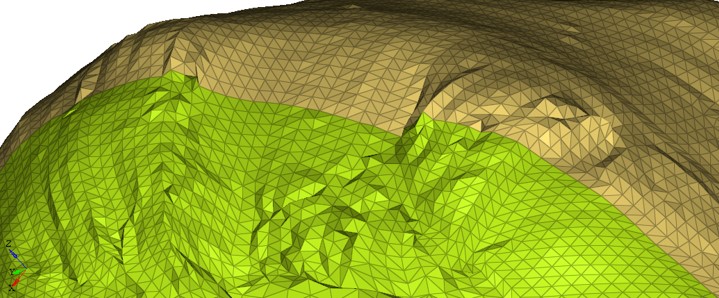
Рисунок 385:

Неправильное граничное условие/начальная скорость

Проверьте, есть ли граничное условие, примененное к баллону подушки безопасности. В моделировании саней/полного транспортного средства это может помешать подушке безопасности двигаться вместе с транспортным средством. Эти граничные условия могут исходить из другой модели моделирования подушки безопасности.

При запуске случая саней с начальной скоростью не забудьте проверить, что подушка безопасности включена. Хорошей практикой в ​​этом случае является изолировать транспортное средство и убедиться, что все узлы имеют начальную скорость > 0 при t=0.

Внутренние узлы в деталях с материалами VOID

Детали, которым назначен материал void, не должны иметь никаких внутренних узлов, поскольку материал VOID не имеет жесткости. Материал void иногда используется для определения поверхностей связи или вентиляционных отверстий.

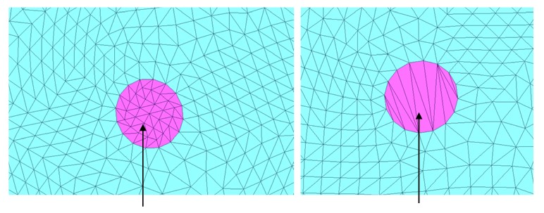
Рисунок 386: Слева: Материал пустоты без внутренних узлов; Справа: Неправильный материал пустоты имеет внутренние узлы

Неправильная ориентация нормали

Для контролируемого объема нормаль всех сегментов, определяющих поверхность, должна указывать наружу. В противном случае решатель выведет сообщение об ошибке в выходном файле Starter.

 ИДЕНТИФИКАТОР ОШИБКИ: 8
 ** ОШИБКА В ОПРЕДЕЛЕНИИ КОНТРОЛИРУЕМОГО ОБЪЕМА
 ОПИСАНИЕ:
     --ИДЕНТИФИКАТОР КОНТРОЛИРУЕМОГО ТОМА: 6620000
     --НАЗВАНИЕ КОНТРОЛИРУЕМОГО ТОМА :       PAB
ОТКРЫТЫЙ ОБЪЕМ ИЛИ НЕПРАВИЛЬНАЯ ОРИЕНТАЦИЯ ЭЛЕМЕНТА

РЕШЕНИЕ :

ОБЪЕМ ДОЛЖЕН БЫТЬ ЗАКРЫТ, А НОРМАЛИИ ОРИЕНТИРОВАНЫ НАРУЖУ

Проверьте нормаль элементов, которые определяют контролируемый объем в HyperCrash или HyperMesh и отрегулируйте соответствующим образом.

Примечание: Если ссылочная геометрия определена с помощью``/EREF``, изменение нормали элементов может быть опасным, поскольку это создаст разрыв между связностью элементов в ссылке и сложенной/масштабированной сетке.

Вместо изменения нормали элементов, лучшим решением будет попросить решатель обратить нормаль при генерации поверхности определенного компонента.

В примере ниже решатель обратит нормаль ID детали = 1.

/SURF/PART/19

Подушка безопасности -1 2 3 5 8 9

Временной шаг подушки безопасности, /DT/FVMBAG/1

В файле Engine должна присутствовать обработка временного шага /DT/FVMBAG/1.

Например:

/DT/FVMBAG/1
0.9 0.0002
/FVMBAG/MODIF
#monvol_ID
2000
#  igmerg  cgmerg  cnmerge  ilvout
1  0.01000  0.001000  1

Статический тест раскрытия

Перед применением модели подушки безопасности в модели вашего автомобиля рекомендуется сначала запустить статический тест раскрытия.

Для этого теста используйте:

• Параметры файла шага времени Engine (/DT/NODA/CST; /DT/INTER/DEL, …), которые вы будете использовать в полной симуляции автомобиля/саней

• Версию решателя, которую вы будете использовать в полной симуляции автомобиля/саней

Убедитесь, что подушка безопасности раскрывается правильно. Проверьте добавленную массу, объем, давление, массу газа и массу выходящего газа, чтобы убедиться, что подушка безопасности раскрывается, как ожидается. Если подушка безопасности не раскрывается, как ожидается, маловероятно, что она сможет раскрыться хорошо в полной симуляции автомобиля.

Руководство по отладке

Модели автокатастроф обычно сложны с большим количеством элементов, материалов, свойств, пружин, интерфейсов и т. д. Если полученные численные результаты не соответствуют физическому поведению или если вычисление останавливается с сообщениями об ошибках, не всегда легко найти источник проблемы моделирования. Необходим метод проверки моделей при возникновении проблем.

Следующие рекомендации помогают исправить большинство проблем; но не все из них. Сложные модели с упрощающими предположениями моделирования трудно исправить, и для них требуется опытный пользователь.

Потенциальные проблемы в сложных моделях можно отслеживать и решать в три шага:

• Перед вычислением

• После компиляции PRADIOS Starter

• Во время или после вычислений с помощью постпроцессоров

В следующих разделах описывается метод отладки.

Подготовка модели

Специализированные инструменты препроцессора Laduga для интеграции большого количества контроллеров моделей. Эти инструменты также включают в себя автоматические алгоритмы коррекции. Наиболее распространенные проверки перед запуском модели связаны с:

• Качество сетки

• Определение пружины

• Пересечения и проникновения в определение интерфейса

• Проверка несовместимых кинематических условий:

  ◦ Нет общих вторичных узлов между твердыми телами

  ◦ Только «свободный» главный узел

  ◦ Сферическая инерция для малых

• Масса и центр тяжести

• Толщина деталей

• Начальное значение скорости и направление

• Нормаль жесткой стенки

• Закон материала: согласованность системы единиц

• Свободные узлы

• Контролируемый объем:

◦ Закрытый объем

◦ Положительный объем

• Связность между частями

• Размеры сетки между соединенными частями

Представлены некоторые основные правила создания допустимой модели.

Качество сетки

Рекомендации по сетке, обсуждаемые в разделе «Конечные элементы», следует соблюдать. Сетка оболочки должна быть максимально однородной. Не рекомендуется использовать разные формулы оболочки для данной физической детали. Для очень мелких сеток рекомендуется использовать полностью интегрированные элементы или метод физической стабилизации (/PROP/SHELL). Треугольные оболочки избегаются. Если сетка включает треугольники из-за сложной сетки, рекомендуется уменьшить их количество до 5% на деталь.

Проверка материала

Некоторые распространенные вопросы по проверке материала: 1. Материал находится в правильной системе единиц??

• Для металлических деталей:

40 GPa < Modulus < 210 GPa

1.8e-6 kg/mm³ < Плотность < 7.8e-6 kg/mm³

• Для пластиковых деталей (PP, PC-ABS, PP GF30%…):

0.9 GPa < Modulus < 13 GPa

9e-7 kg/mm³ < Плотностьy < 1.6e-6 kg/mm³

• Для пены:

1e-8 kg/mm³ < Плотность < 1e-7 kg/mm³

2. Это проверенный материал из базы данных материалов?

   Необходимо ввести реалистичные данные о материалах.

3. Проверьте наличие этих распространенных проблем в материале.

   • Отрицательные наклоны на кривой напряжение-деформация

   • Эластичный материал назначается деформируемым деталям

   • Нереалистичный предел текучести (> 2 ГПа)

   • Разрушение не определено, а элементы пластиковых или металлических деталей растягиваются нереалистично (пластическая деформация > 1)

Некоторые из упомянутых выше проверок можно выполнить в HyperCrash.

• Согласованность агрегата можно проверить с помощью проверки контура на панели качества.

• Проверка «Деталь не интегрирована в rbody для LAW1» находит детали, которые деформируются и используют материал LAW1, который может стать нестабильным,

если деформация станет большой.

Рисунок 387:

Определение твердого тела и оболочки

Для некоторых материалов рекомендуется использовать специальную опцию в оболочке или твердом теле.

1. Для деталей, использующих упругопластический закон материала (LAW2, LAW27, LAW36 и т. д.).

   • \(I_{shell} =24, I_{smstr} =4, I_{plas} =1, I_{thick} =1, N =5\)

2. Для твердых деталей с использованием закона упругопластического материала (LAW2, LAW27, LAW36, etc.).

   • Для гексаэдрических элементов: \(I_{solid} =24, I_{smstr} =4\)

   • Для тетраэлементов первого порядка: \(I_{solid} =1, I_{tetra}\) =0 или 1

   • Для тетраэлементов второго порядка: \(I_{solid}\) =1

3. Для твердых деталей с использованием гиперэластичного материала (LAW42, LAW69, etc.)

   • Для шестигранных элементов: \(I_{solid} =24, I_{smstr} =10, I_{cpre} =1, I_{HKT} =2\)

   • Для тетраэлементов: \(I_{solid} =1, I_{smstr} =10\)

4. Для пены:

   • Материал LAW38: \(I_{solid} =24, I_{smstr} =10\)

   • Материал LAW70: \(I_{solid}\) =1 or 17, \(I_{smstr}\) =1 or 11

   • Для пенопласта, смоделированного с помощью тетраэлементов, \(I_{tetra}\) не следует устанавливать значение 1, так как пена очень сжимаема.

5. Для ткани:

   • LAW19 триа-элементы: \(I_{shell} =4, I_{smstr} =1, d_{m} =0.2, N =1\)

   • LAW58 триа-элементы: \(I_{shell} =4, I_{smstr} =4, d_{m} =0.2, N =1\)

Это также можно проверить с помощью HyperCrash Model Checker.

Рисунок 388: LAW70

Рисунок 389: LAW42

Определение пружины

Нефизическое или плохое определение пружин является распространенной проблемой в моделях столкновений. Фактически, свойства пружин должны быть согласованы по массе, инерции, жесткости и длине. Фактически, пружина должна иметь физическое поведение:

• Что касается распределения массы по одномерному стержню, то инерция будет иметь верхний и нижний пределы:

\[\frac{ml^{2}}{12}\leq I\leq\frac{ml^{2}}{4}\tag{280}\]

Нижний предел — это инерция равномерно распределенного стержня. Верхний предел дает инерцию стержня с двумя крайними массами m/2. Поскольку пружины также используются для моделирования болтов и точечной сварки, вы можете выйти за эти ограничения и записать:

\[ \begin{align}\begin{aligned}0.0ml^{2}\leq I\leq 100ml^{2}\tag{281}\\- Поперечное сечение пружины можно вычислить либо с помощью :math:`S=\frac{Kl}{E}, либо S=\frac{m}{\rho l}`. Если отношение между двумя вычисленными значениями больше 100, несоответствие может привести к некоторым проблемам.\\- В свойствах пружины для отрицательной деформации сила должна быть отрицательной, а для положительной деформации - положительной. В противном случае пружина генерирует энергию во время вычисления.\\- Если касательная жесткость отрицательна для нелинейной упругой пружины, существует риск неустойчивости, особенно при вибрации в зоне отрицательного наклона (энергетическая ошибка может стать положительной и увеличиться).\\- Если максимальный наклон кривой (то есть максимальная жесткость) больше начальной жесткости, разгрузка в зоне максимального наклона будет ложной (см. Инструменты моделирования).\\- Очень высокая жесткость в элементах пружины может привести к низкому временному шагу и неустойчивости.\end{aligned}\end{align} \]

Например, следующая проверка в HyperCrash позволяет выявить пружинный элемент, имеющий необычно высокую жесткость при растяжении (1000 кН/мм) и вращении (10000 кН.мм/рад).

Примечание: Свойство, на которое есть ссылки в частях фиктивных / барьерных моделей, следует игнорировать.

Рисунок 390:

Согласованность пучка

В дополнение к предположению длины/глубины пучка > 10, следующие рекомендации определяют согласованность пучка:

\[L>\sqrt{A}\tag{282}\]

\(0.01A^{2}<I_{y}<100A^{2}\)

\(0.01A^{2}<I_{z}<100A^{2}\)

\(0.1\left(I_{y}+I_{z}\right)<I_{x}<10\left(I_{y}+I_{z}\right)\)

Пересечения и проникновения в интерфейсах

Начальные пересечения сетки создают нереалистичные соединения. Более того, это может привести к ситуациям блокировки, ведущим к сбою вычислений.

Начальные проникновения обусловлены определением зазора интерфейса. Они приводят к нереалистичным и неконтролируемым внутренним силам, которые могут вызвать локальные пластические деформации в начале вычислений. Структура затем локально менее жесткая.

Инструменты препроцессора Laduga можно использовать для обнаружения и удаления пересечений и начальных проникновений. Модель, содержащая много начальных проникновений, не может считаться допустимой. После исправлений, если остается несколько начальных проникновений, флаг Inacti =1 можно активировать в /INTER/TYPE7. В этом случае жесткость интерфейса для первоначально пройденных узлов деактивируется.

Если остаются только небольшие начальные проникновения (менее 5% от зазора), можно использовать переменный зазор во времени, установив флаг Inacti=5; что лучше, чем Inacti=1.

• Лучшая практика (рекомендуется):

  ◦ Для интерфейса TYPE7, 11 и 19:

  ∙ \(I_{stf} =4, St_{min} = 1, I_{del}\) = 1 or 2, \(I_{nacti} =6, I_{form} =2, Gap_{min} ≥ 0.49\)

  ∙ В областях, где моделирование не удается, нет пересечения

  ∙ Проникновения не слишком глубокие (проверьте остаточное расстояние в HyperCrash/HyperMesh). Оно не должно быть ниже 0.1mm.

  ◦ Для интерфейса TYPE2:

  ∙ Используйте \(Spot_{flag}\) = 28, если основной узел является оболочкой или вторичный узел имеет вращательную степень свободы, а основной — нет (сплошной)

  ∙ Используйте \(Spot_{flag}\) = 27, если и вторичный, и основной не имеют вращательной степени свободы (сплошной) \(I_{del}\) следует установить на 1 для всех случаев

Определение жесткого тела

Следует отметить следующие рекомендации:

• Никогда не используйте узел сетки в качестве основного узла для твердого тела

• Твердое тело, состоящее из двух вторичных узлов, требует использования флага сферической инерции (\(I_{spher}\) =1 в /RBODY)

• Помните, что основной узел может перемещаться при инициализации твердого тела в PRADIOS Starter

Большинство проблем определения твердого тела можно обнаружить и исправить с помощью инструментов препроцессора Laduga.

Несовместимые кинематические условия

Несовместимые условия могут привести к увеличению общей энергии и невоспроизводимости результатов в параллельных вычислениях, даже если /PARITH/ON используется. PRADIOS Starter обнаруживает потенциальные несовместимые условия, которые должны контролироваться вами.

Параллельные вычисления

Опция /PARITH/ON должна использоваться при использовании многопроцессорных систем. Если она не используется, проблемы будет трудно воспроизвести, и они могут появляться и исчезать.

Комментарии

1. Использование Inacti =1 делает модель более мягкой.

2. Никогда не помещайте свободные узлы в интерфейсы. Выбор поверхностей в определении интерфейса должен выполняться с помощью оболочек и твердых элементов (или частей), а не узлов.

Согласованность единиц

В PRADIOS могут быть предоставлены данные для любой системы единиц, но очень важно сохранить согласованность единиц. Если модель не имеет согласованности единиц, это приведет к неверным результатам (неожиданному поведению) или может привести к ошибке в расчетах.

Основные единицы

	SI			CGS	Hydro	US	Japan ese
Длина	m	mm	mm	cm	cm	in	mm
Масса	kg	Mg (Ton)	kg	g	g	lb	kg
Время	s	s	ms	s	µs	s	ms
Плоский угол	rad	rad	rad	rad	rad	rad	rad
Темпе ратура	K	K	K	K	K	K	K
Частота	Hz	Hz	Hz	Hz	Hz	Hz	Hz
Грави тация	9.81	9.8 1E+03	9.8 1E-03	9.8 1E+02	9.8 1E-10	386	9.8 1E-03

Пример единицы СИ

Длина

[m]

Масса

[kg]

Время

[s]

Угол плоскости

[rad]

Температура

[K]

Частота

[Hz]

Скорость вращения

\(\big{[}\frac{rad}{s}\big{]}\)

Площадь

\([m^{2}]\)

Объем

\([m^{3}]\)

Момент площади (инерция)

\([m^{4}]\)

Расход

\([м^{2}]\)

Скорость

\(\big{[}\frac{m}{s}\big{]}\)

Ускорение

\(\big{[}\frac{m}{s^{2}}\big{]}\)

Натяжение

\(\big{[}\frac{m}{s}\big{]}\)

Линейная масса

\(\big{[}\frac{kg}{m}\big{]}\)

Поверхностная масса

\(\big{[}\frac{kg}{m^{2}}\big{]}\)

Объемная масса

\(\big{[}\frac{kg}{m^{3}}\big{]}\)

Масса поток

\(\big{[}\frac{kg}{s}\big{]}\)

Объем потока

\(\big{[}\frac{m^{3}}{s}\big{]}\)

Количество движения

\(\big{[}\frac{kg\cdot m}{s}\big{]}\)

Кинетический момент

\(\big{[}\frac{kg\cdot m}{s}\big{]}\)

Момент инерции (l)

\(\big{[}kg\cdot m^{2}\big{]}\)

Момент силы

\(\big{[}N\cdot m^\big{]}\)

Сила

\(\big{[}N\big{]}\)

Линейная сила

\(\big{[}\frac{N}{m}\big{]}\)

Жесткость

\(\big{[}\frac{N}{m}\big{]}\)

Вращательная жесткость

\(\big{[}\frac{N\cdot m}{rad}\big{]}\)

Вращательное демпфирование

\(\big{[}\frac{N\cdot m\cdot s}{rad}\big{]}\)

Демпфирование кручения

\(\big{[}\frac{kg\cdot m^{2}}{s\cdot rad}\big{]}\)

Вязкое демпфирование

\(\big{[}\frac{kg}{s}\big{]}\)

Демпфирование изгиба

\(\big{[}\frac{N\cdot s}{m}\big{]}\)

Квадратичная объемная вязкость

\(\big{[}\rho\alpha^{\lambda}\cdot s\big{]}\)

Динамическая вязкость

\(\big{[}Pa\cdot s\big{]}\)

Кинематическая вязкость

\(\big{[}\frac{m^{2}}{s}\big{]}\)

Плотность

\(\big{[}\frac{kg}{m^{3}}\big{]}\)

Мощность

\(\big{[}W\big{]}\)

Энергия

\(\big{[}J\big{]}\)

Энтальпия

\(\big{[}J\big{]}\)

Энтропия

\(\big{[}\frac{J}{K}\big{]}\)

Скорость деформации

\(\big{[}\frac{1}{s}\big{]}\)

Время релаксации

\(\big{[}s\big{]}\)

Тепловое расширение

\(\big{[}\frac{1}{K}\big{]}\)

Теплопроводность

\(\big{[}\frac{W}{m\cdot K}\big{]}\)

Тепловое сопротивление

\(\big{[}\frac{W}{m^{2}\cdot K}\big{]}\)

Удельная теплоемкость (Cp, Cv)

\(\big{[}\frac{kg}{s^{2}\cdot m\cdot K}\big{]}\)

Удельная теплоемкость (Cp)

\(\big{[}\frac{J}{m^{3}\cdot K}\big{]}\)

Проверка согласованности

Используйте основные единицы измерения Масса, Длина или Время, чтобы вы могли получить все остальные необходимые вам единицы.

\(Сила = Масса \cdot Ускорение = \frac{Масса\cdot Длина}{Время^{2}}\)

\(Давление = \frac{Сила}{Площадь} = \frac{Масса}{Длина\cdot Время^{2}}\)

\(Энергия = Сила\cdot Длина\frac{Масса\cdot Длина^{2}}{Время^{2}}\)

\(Плотность = \frac{Масса}{Объем} =\frac{Масса}{Длина^{3}}\)

\(Ускорение = \frac{Длина}{Время^{2}}\)

\(Объем = Длина^{3}\)

Например, использование базовой единицы [кг], [мм] или [мс] даст следующие единицы силы, давления или Судьбы.

\(Сила = \frac{Масса\cdot Длина}{Время^{2}}=\frac{[кг]\cdot [мм]}{[мс]^{2}}=10^{3}\frac{[кг]\cdot [м]}{[с]^{3}}=[кН]\)

\(Давление = \frac{Масса}{Длина\cdot Время^{2}}=\frac{[кг]}{[мм]\cdot [мс]^{2}}=10^{9}\frac{[кг]}{[м]\cdot [с]^{2}}=[ГПа]\)

\(Энергия = \frac{Масса\cdot Длина^{2}}{Время^{2}}=\frac{[кг]\cdot [мм]^{2}}{[мс]^{2}}=\frac{[кг]\cdot [м]^{2}}{[с]^{2}}=[Дж]\)

\(Плотность =\frac{Масса}{Длина^{3}}=\frac{[кг]}{[мм]^{2}}=10^{6}\cdot\frac{[кг]}{[м]^{2}}\)

Проверьте единицы измерения

Карточка свойства

проверьте единицу толщины в свойстве, если это оболочка

Карточка материала

проверьте единицу плотности, проверьте модуль упругости, проверьте единицу напряжения, если возможно

Нагрузка

проверьте единицу силы, проверьте единицу тяжести, если используется /GRAV

Длина

измерьте единицу длины геометрии с помощью HyperCrash или HyperMesh

Все единицы должны быть согласованы.

Самые популярные единицы (с примерами из стали)

Масса	Длина	Время	Сила	Энергия Янга	стресс	стресс Плот ность	модуль	Грави тация	Урожай
kg	m	s	N	J	Pa	7.8 e+03	2.1 e+11	9 .81e +00	2 .06e +05
g	mm	ms	N	mJ	MPa	7.8 e-03	2.1 e+05	9.81 e-03	2 .06e +02
kg	mm	ms	KN	J	GPa	7.8 e-06	2.1 e+02	9.81 e-03	2.06 e-01
Mg (ton)	mm	s	N	mJ	MPa	7.8 e-09	2.1 e+05	9 .81e +03	2 .06e +02
g	cm	micros	\(10 ^{7}\) N	\(10 ^{5}\) J	Mbar	7.8 e+00	2.1 e+00	9.81 e-10	2.06 e-06

Инструментарий модели

Выходные данные и частоты хранения должны быть установлены для получения достаточной информации для результатов постобработки.

Переменные для сохранения

Чтобы найти источник проблем, вам нужны выходные файлы с достаточной информацией, особенно для наиболее потенциально проблемных объектов, таких как пружины, интерфейсы и жесткие тела.

Пружины

сохранить все элементы пружин и балок (кроме пружин точечной сварки) /TH/SPRING Измерить смещения и силы внутри определенной пружины Пример: опора двигателя, подрамник, фиксация и т. д.

nterfaces

сохранить все контактные интерфейсы (кроме ТИПА 2) /TH/INTER Вывести силы определенных интерфейсов Пример: манекен/ремень

Rigid Bodies

измерить смещения и силы внутри определенных жестких тел Пример: фиксации подрамника, опора двигателя и т. д.

Section, Rigid Wall и Monitored Volume

сохранить все выходные данные TH

Настройте движок PRADIOS на сохранение переменных в файлах анимации:

Масса

/ANIM/MASS

Узловое изменение массы

/ANIM/NODA/DMAS

Пластическая деформация

/ANIM/ELEM/EPSP

фон Мизес

/ANIM/ELEM/VONM

Песочные часы

/ANIM/ELEM/HOURG

Удельная энергия

/ANIM/ELEM/ENER

Скорость

/ANIM/VECT/VEL

Контакты

/ANIM/VECT/CONT

Сила на жесткой стенке

/ANIM/VECT/FOPT

Кроме того, /ANIM/VECT/ACC и /ANIM/VECT/FINT могут быть полезны в случае возникновения проблемы.

Примечание: Обязательно получите файл анимации, если запуск не удается; вы можете использовать опцию /STOP в файле Engine. Если вычисление останавливается, выполните еще один перезапуск и запишите анимацию в первом цикле.

Проверка модели с помощью PRADIOS Starter

PRADIOS Starter проверяет соответствие между строками формата и выдает ошибки и предупреждения, если они есть. Выходной файл runname_0000.out содержит полезную информацию, помогающую отлаживать модели.

Следующие проверки полезны в выходном файле:

Сообщения об ошибках и предупреждениях

Все ошибки должны быть исправлены. Предупреждение, требующее исправления:

• Вырожденные элементы

• Начальные проникновения

• Реальные несовместимые кинематические условия

Проверьте шаг времени (элемент и узел)

сколько элементов контролируют временной шаг? Если несколько, то измените сетку, чтобы оптимизировать временной шаг.

Проверьте массу и инерцию

Масштабирование массы вызывает нестабильность. Стоит проверить центр тяжести, вычисленный PRADIOS. Он должен соответствовать физическому центру тяжести.

Примечание: Мелкие элементы, балки, пружины и точечные сварные швы требуют тщательного наблюдения.

Проверка вычислений

Это метод проверки качества результатов моделирования. Даже если прогон не дает сбоев, необходимо проверить, что соблюдаются три фундаментальных закона сохранения. Изменение шага по времени и качественная оценка результатов могут помочь избежать ошибок моделирования.

Баланс энергии

С учетом внешних работ общая энергия должна оставаться постоянной или немного уменьшаться. Общая энергия может увеличиваться в конце вычисления, во время возврата или в начале во время первых циклов.

Внутренняя энергия + Кинематическая энергия + Энергия песочных часов + Энергия контакта + … = Изменение внешней работы

Если используются недоинтегрированные элементы, общая энергия песочных часов должна оставаться ниже 10% от общей энергии. Если это не так, сетку следует переработать или использовать элементы с методом физической стабилизации.

Энергия контакта на самом деле не является физической. Для каждого подмножества и для каждой части рекомендуется следующее ограничение:

\[\frac{E_{h}+E_{c}}{E_{t}}\leq 15%\tag{283}\]

Где,

\(E_{h}\) Энергия песочных часов

\(E_{c}\) Контактная энергия

\(E_{t}\) Общая энергия

Ошибка энергии вычисляется PRADIOS как:

\[%Error=100\left(\frac{E_{k}+E_{k}^{r}+E_{i}}{E_{k,1}+E_{k,1}^{r}+E_{i,1}+E_{wk}-E_{wk,1}}-1\right)\tag{284}\]

Где,

\(E_{k}\) Поступательная кинетическая энергия

\(E_{k}^{r}\) Вращательная кинетическая энергия

\(E_{ih}\) Внутренняя энергия

\(E_{wk}\) Внешняя работа

\(E_{k,1}\) Начальная поступательная кинетическая энергия

\(E_{k,1}^{r}\) Начальная вращательная кинетическая энергия

\(E_{i,1}\) Начальная внутренняя энергия

\(E_{wk,1}\) Начальная внешняя работа

Ошибка должна быть отрицательной и уменьшающейся (за исключением первого цикла или на этапе отскока). Ошибка должна быть менее 15% в конце вычисления (5% для хорошей модели). Если ошибка немного увеличивается, то уменьшение может быть нормальным. Если ошибка увеличивается, это означает, что возникла проблема. Затем ошибка может вырасти до 99,9% с сообщением об ошибке вычисления.

Баланс массы

Если масса увеличивается, ее изменение должно оставаться менее 1% для каждого подмножества и для каждой части \(\big{(}\frac{dM}{M}\) <1%. Если изменение массы составляет от 1% до 3%, проверьте, движутся ли узлы с добавленной массой или нет. Если это так, добавленная масса приводит к увеличению кинетической энергии. Для более чем 3% изменения, результаты, вероятно, плохие.

Баланс импульса

Динамическое равновесие каждого узла удовлетворяется законом Ньютона в конце каждого цикла. Поскольку PRADIOS решает уравнения равновесия в каждом цикле, обычно баланс импульса удовлетворяется. Однако в случае возникновения проблемы перекрестная проверка между узловыми ускорениями и силами удара (интерфейс, жесткая стенка, барьер и т. д.) может помочь лучше понять проблемы.

\[F_{wall}=\dfrac{M\text{onenturmariation}}{dt}\tag{285}\]

Эволюция временного шага

Если временной шаг уменьшается, а затем быстро увеличивается, то проблемы нет. Если он сильно меняется от одного цикла к другому, это может быть связано с жесткостью интерфейса.

Если временной шаг остается низким, возникла проблема. В этом случае найдите узел (или элемент), контролирующий временной шаг, и попытайтесь понять, почему произошло уменьшение.

Визуальный осмотр деформированных деталей

После получения некоторых файлов анимации общую деформацию структуры можно сравнить с физическим поведением. Осмотрите деформированную форму, чтобы убедиться:

• Нет летящих узлов (частей)

• Деформированная форма гладкая

• гол хорды между соседними элементами достаточно мал

• Нет пересечений

Хорошее физическое поведение достигается, когда:

• Пластическая деформация составляет менее 30%

\[\dfrac{E_{k}+E_{k}^{r}}{E_{t}}\leq 1%\]

Бессмысленные результаты

Контактные силы, напряжение по Мизесу, узловые скорости и ускорения должны быть тщательно проверены. Если значения бессмысленны (например: напряжение по Мизесу = 1 ГПа), первой проверкой может быть согласованность системы единиц. Более подробную информацию см. в Приложении.

См. также

Проверка результатов (FAQ)

Отладка модели

Вот несколько рекомендаций по поиску источника проблем с вычислениями.

Во-первых, обратите внимание, что PRADIOS Explicit Solver позволяет решать высоконелинейные динамические задачи; вычисление может быть неверным, даже если запуск не завершится. Если вычисление доходит до конца, оно иллюстрирует хорошее численное поведение, но не обязательно хороший физический ответ. Однако, необходимо получить сообщение "Нормальное завершение" в конце выходного файла Engine, чтобы проверить процедуры численного разрешения.

Достоверность результатов может быть продемонстрирована путем выполнения следующих условий:

• Числовая устойчивость

• Физическое поведение

• Физическая надежность

Численная устойчивость обеспечивается, если сообщение "Нормальное завершение" и проверены баланс энергии и массы.

Если подготовленная модель на самом деле не отражает физическую проблему, могут быть получены неправильные результаты. Чтобы понять проблему, сначала нужно задать хорошие вопросы, на которые следует ответить, чтобы доказать надежность результатов:

• Насколько результат зависит от трения?

• Насколько модель зависит от явлений разрыва?

• Насколько результат зависит от неизвестных параметров материала?

• Насколько модель зависит от других явлений, которые трудно моделировать?

Если результаты сильно зависят от заданного параметра, необходимо провести экспериментальное испытание, чтобы использовать высокоточные значения для вычислений.

Примечание: Лучшей моделью является та, для которой вы знаете значения физических параметров!

Расхождение

Расхождение происходит, когда наблюдается одно из следующих условий:

• Положительная ошибка энергии (кроме первого цикла)

• Отрицательная ошибка энергии более чем на 15% (кроме первого цикла)

• Активация кинематического временного шага в интерфейсе TYPE7

• Временной шаг, заданный твердым телом

• Необъяснимые изменения временного шага

• Быстрое увеличение массы

Существует три типа расхождения:

Быстрое расхождение

Увеличение ошибки энергии часто экспоненциально. Расчет не удается в нескольких циклах. Возможные причины:

• Несовместимые кинематические условия

• Отрицательная жесткость в пружине

• Отрицательная жесткость в табличном законе материала

• Вторичные узлы слишком далеко от основной поверхности в интерфейсе TYPE2

Поздняя дивергенция

Временной шаг слишком мал. Структура искажена и наблюдаются высокие проникновения во многие интерфейсы.

Возможная причина — качество сетки

Медленное расхождение

Конечная ошибка не обязательно является причиной расхождения. Возможные причины:

• Для линейного отклонения причиной может быть наличие несовместимых кинематических условий.

• Для синусоидального отклонения это обычно освобожденная или генерируемая энергия (пример: начальные проникновения и функции жесткости пружины).

• Слишком мягкий материал также может быть причиной.

Если важно найти, какое событие вызвало проблему. Необходимо проверить событие прямо перед расхождением. Если для данной части наблюдается странное поведение, то также необходимо изучить связанные части и предыдущие события.

Проблемы с запуском

Запуск останавливается на цикле 0

Данные не записаны в выходной файл Engine runname_0001.out. Обычно это происходит из-за неправильной процедуры запуска, когда файл Restart не может быть правильно прочитан.

Работа останавливается после нескольких циклов

Данные записываются в выходной файл Engine runname_0001.out.

Источником проблемы могут быть несовместимые кинематические условия (например: жесткие тела с общим вторичным узлом) или значения, выходящие за пределы границ свойств материала или элемента; хотя, причиной могут быть начальные проникновения.

Выполнение останавливается во время вычисления

Сначала проверьте необходимое дисковое пространство, затем можно изучить поведение непосредственно перед и после расхождения. Необходимо наблюдать эволюцию временного шага и энергетическую ошибку.

• Файл анимации перед запуском завершается. Это очень полезно для определения областей:

  ◦ Где скорость выходит за пределы диапазона (>> 100 m/s)

  ◦ Масса прибавляется

  ◦ Деформация чрезмерна (проверьте пластическую деформацию))

  ◦ Напряжение нереалистично (> 2 ГПа))

  В HyperView просмотрите анимацию и визуально проверьте наличие очевидных проблем:

  ∙ Скорость не применяется ко всем узлам транспортного средства.

  ∙ Неправильные граничные условия

  ∙ Отсутствующие соединения (ремень безопасности не подключен должным образом и т. д.)

  ∙ Просмотрите основные контуры:

  1. Стресс по Мизесу: проверка значений, выходящих за пределы

  2. Добавленная масса: проверьте на очень большую массу

  3. Скорость: проверьте на очень большую скорость Во многих случаях узлы с самой высокой скоростью или большой добавленной массой будут находиться в одной области.

• Точка в файле T01. Это полезно для определения:

◦ Часть, которая имеет внезапное увеличение внутренней/кинетической энергии. Постройте график внутренней и кинетической энергии всех частей в HyperGraph (вам необходимо поместить все части в историю времени).

◦ Постройте график глобального энергетического баланса, чтобы определить, вызвано ли расхождение внутренней энергией, кинематической энергией, внешней рабочей силой.

• Информация в конце файла листинга (_0001.out).

  Например, в приведенном ниже случае информация, представленная в конце _0001.out, очень полезна для понимания области модели, вызывающей остановку моделирования.

  Решатель сообщает:

  ◦ Какие части имеют самую высокую кинетическую (1) / внутреннюю энергию (2)

  ◦ Какие узлы имеют самую высокую скорость (3) / изменение массы (4)

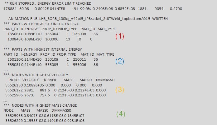
Рисунок 391:

Например, в приведенном ниже случае, перед тем как симуляция завершится ошибкой в файле ``_0001.out` может быть напечатано следующее сообщение`:

ВРЕМЯ ЦИКЛА ВРЕМЯ-ШАГ ЭЛЕМЕНТ ОШИБКА I-ЭНЕРГИЯ K-ЭНЕРГИЯ T K-ENERGY R EXT-WORK MAS.ERR 62100 18.53 0.2985E-03 SOLID 230440718 -1.3% 0.3484E+05 0.1313E+06 109.7 1523. РАЗРЫВ ТВЕРДОГО ЭЛЕМЕНТА НОМЕР 230025298 УДАЛИТЬ СОЕДИНЕНИЕ ТВЕРДЫЙ ЭЛЕМЕНТ 110010956, ENERGY= 4.732011155E-05 РАЗРЫВ ТВЕРДОГО ЭЛЕМЕНТА НОМЕР 230024559 **ПРЕДУПРЕЖДЕНИЕ МИНИМАЛЬНЫЙ ШАГ ВРЕМЕНИ 0.5976E-05 В ИНТЕРФЕЙСЕ NB 2300040(DTMIN= 0.1000E-04) ВТОРИЧНЫЕ УЗЛЫ NB 230373002 230373019 ГЛАВНЫЕ УЗЛЫ NB 230373003 230373004 УДАЛИТЬ ВТОРИЧНУЮ ЛИНИЮ ИЗ ИНТЕРФЕЙСА

Первоначальное пересечение вызывает сильное искажение и в конечном итоге ОШИБКУ завершение.

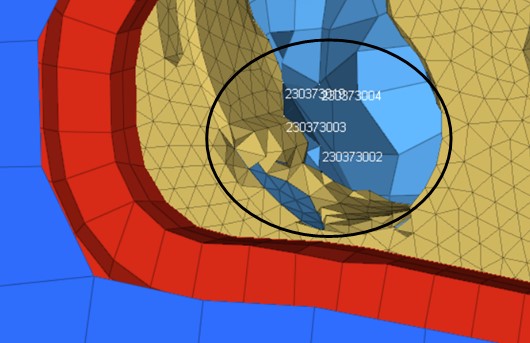
Рисунок 392:

Например, в приведенном ниже случае запуск прекращается из-за контакта с жестким объектом, что приводит к завершению ERROR. Выходной файл выводит:

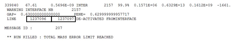
Рисунок 393:

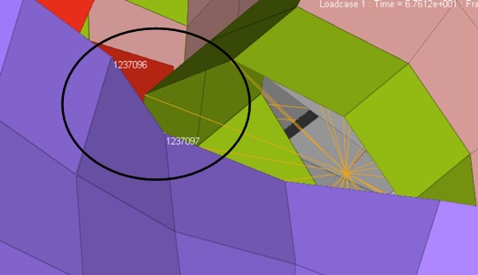
Рисунок 394:

Сообщение об отрицательном объеме

Это в основном из-за высокой деформации сплошных сеток. Полностью интегрированные кирпичные элементы особенно подвержены этой проблеме, которая может быть вызвана плохим поведением интерфейса или плохими определениями материалов. В любом случае рекомендуется использовать формулировку совместного вращения, чтобы избежать плохой реакции на сдвиговую деформацию.

Предположение параметров расчета напряжения и деформации (/PROP) можно использовать с /DT/BRICK/CST, чтобы избежать отрицательных объемов (см. разделы Временной шаг и Конечные элементы для получения более подробной информации об этой опции).

Основные отношения

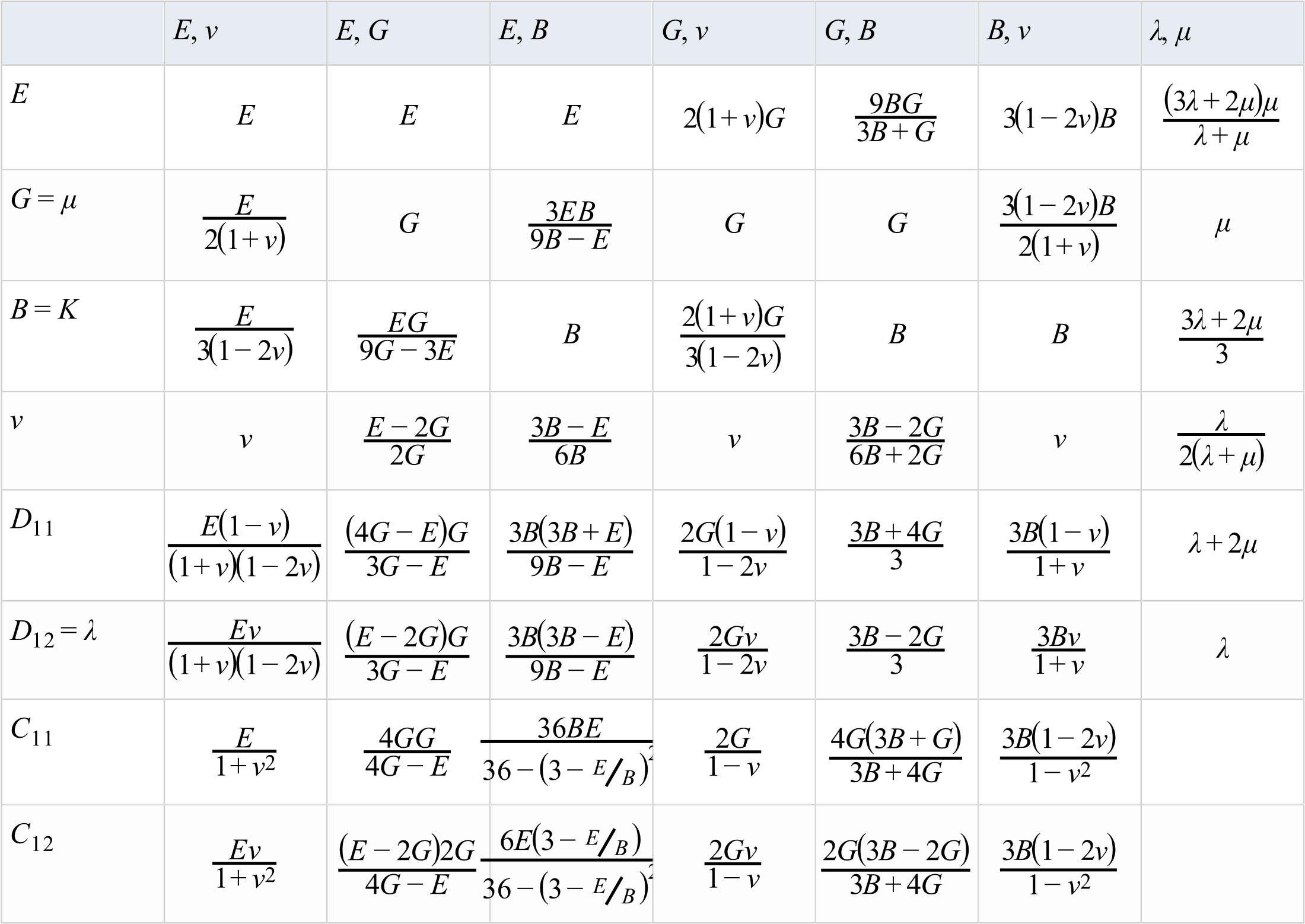
Закон Хука 3D (главное напряжение и деформация)

\(\sigma = Dc\)

\(\sigma_{1} = D_1\varepsilon_{1}+D_12\varepsilon_{2}+D_13\varepsilon_{3}\)

\(\sigma_{1} =(\lambda+2\mu)\varepsilon_{1}+\lambda(\varepsilon_{2}+\varepsilon_{3})\)

\(\sigma_{1} =\lambda(\varepsilon_{1}+\varepsilon_{2}+\varepsilon_{3})+2\mu\varepsilon_{1}\)

\(\sigma_{1} =\varepsilon_{kk}+2\mu e_{1} с \varepsilon_{kk} = \varepsilon_{1}+\varepsilon_{2}+\varepsilon_{3} и e_{1} = \varepsilon_{1} - 1/3 (\varepsilon_{1}+\varepsilon_{2}+\varepsilon_{3})\)

Закон Хука 2D (плоское напряжение)

\(\sigma = C_{11}\varepsilon_{1}+C_{12}\varepsilon_{2}\)

Единичные системы

Длина	Время	Масса	Сила	Давление	Veloc ity	p	“Энергия	G
m	s	Kg	Kg m/s2	N/m2	m/s	Kg/m3	Km g2/s2	9.81
m	s	Kg	N	Pa	m/s	m Kg/l	J	9.81
m	s	g	mN	mPa	m/s	u Kg/l	mJ	9.81
m	s	Mg (ton)	KN	KPa	m/s	Kg/l	KJ	9.81
m	ms	Kg	MN	MPa	Km/s	m Kg/l	MJ	9.8 1e-6
m	ms	g	KN	KPa	Km/s	Kg/l	KJ	9.8 1e-6
m	ms	Mg (ton)	GN	GPa	Km/s	Kg/l	GJ	9.8 1e-6
mm	s	Kg	mN	KPa	mm/s	M Kg/l	mJ	9.8 1e+3
mm	s	g	mN	Pa	mm/s	K Kg/l	nJ	9.8 1e+3
mm	s	Mg (ton)	N	MPa	mm/s	G Kg/l	mJ	9.8 1e+3
mm	ms	Kg	KN	GPa	m/s	M Kg/l	J	9.8 1e-3
mm	ms	g	N	MPa	m/s	K Kg/l	mJ	9.8 1e-3
mm	ms	Mg (ton)	MN	TPa	m/s	G Kg/l	KJ	9.8 1e-3
cm	ms	g	daN	\(10 ^{5}\) Pa bar	dam/s	Kg/l	dJ	9.8 1e-4
cm	ms	Kg	\(10 ^{4}\) N (KdaN)	\(10 ^{8}\) Pa (Kbar)	dam/s	K Kg/l	hJ	9.8 1e-4
cm	ms	Mg (ton)	\(10 ^{7}\) N (MdaN)	\(10 ^{11}\) Pa (Mbar)	dam/s	M Kg/l	\(10 ^{5}\) J	9.81 e-10
cm	u	g	\(10 ^{7}\) N (MdaN)	\(10 ^{11}\) Pa (Mbar)	\(10 ^{4}\) m/s	Kg/l	\(10 ^{5}\) J	9.81 e-10

Фильтрация

Часто бывает полезно отфильтровать результаты в законе материала или разрушения, чтобы удалить численный шум. Наиболее распространенным фильтром является экспоненциальный скользящий средний фильтр. Это особенно важно для моделей материалов, которые включают эффекты скорости деформации.

В большинстве материалов флаг \(F_{smooth}\) = 1 должен быть определен, чтобы включить фильтрацию, а частота среза вводится с помощью \(F_{cut}\). Для случая фильтрации скоростей деформации используйте:

\[\hat{c}_{filtered}(t)=\omega(t)+(1-\alpha)\hat{c}_{filtered}(t-dt)\tag{287}\]

Где,

\(\hat{c}_{filtered}(t)\)

Фильтрованная скорость деформации.

\(\delta(t)\)

Скорость деформации на текущем временном шаге перед фильтрацией.

\(\alpha\)

Степень уменьшения веса, постоянный коэффициент сглаживания от 0 до 1. Более высокое значение быстрее обесценивает предыдущие значения, что приводит к меньшей фильтрации.

\(dt\)

Временной шаг моделирования.

\(\hat{c}_{filtered}(t-dt)\)

Отфильтрованная скорость деформации на предыдущем временном шаге.

Для законов материалов, где можно ввести \(F_{cut}\).

\[\alpha=2\pi dt F_{cut}\tag{288}\]

Где, \(F_{cut}\) - частота среза.

Таким образом,

\[F_{cut}=\frac{\alpha}{2\pi dt}\tag{289}\]

Частота среза является функцией временного шага модели. Опыт показывает, что скорость деформации также важна. Для более медленных скоростей, таких как автомобильная авария, 1–10 кГц (1000–10 000 Гц) является хорошим значением, но для высокоскоростных событий, таких как баллистика, следует использовать меньшую фильтрацию, поэтому 1–10 ГГц подходит. Следует использовать хорошее инженерное суждение для определения разумного значения для каждого моделирования. См. RD-E: 1102 Влияние скорости деформации для примера фильтрации скорости деформации.

В PRADIOS вам доступны как неявные, так и явные схемы интегрирования по времени. В явной схеме скорости и смещения получаются путем прямого интегрирования узловых ускорений. При таком подходе шаг времени цикла часто мал из-за соображений устойчивости. Поэтому для статических или медленных динамических вычислений, где продолжительность исследования велика, для выполнения моделирования требуется много циклов. Альтернативой явному методу в таких случаях является неявная схема интегрирования по времени. Можно показать, что неявная схема безусловно устойчива, что приводит к большему шагу времени цикла по сравнению с явным методом. Однако в неявной схеме глобальная матрица жесткости должна быть собрана и инвертирована, что приводит к более высокой стоимости и большим требованиям к памяти на шаг нагрузки.

Явный подход более привлекателен для быстрых динамических задач с высокой нелинейностью геометрических и материальных характеристик. Поскольку все величины можно рассматривать как векторы, требуется мало памяти. Число циклов для достижения симуляции может быть довольно большим, но глобальная эффективность обычно наблюдается. Неявный метод, с другой стороны, более эффективен для статических приложений и/или длительных симуляций.

Оптимальным решением является наличие как неявных, так и явных методов, легко доступных в одном коде. Кроме того, неявные и явные решатели в PRADIO используют одни и те же процедуры для вычисления внутренней силы, что позволяет плавно переключаться между двумя схемами, без проблем с дисбалансом во время перехода. Поэтому две схемы можно объединить для выполнения многоэтапного анализа. Два варианта использования неявного решения — это пружинение (неявное) после формовки листового металла (явное) или вычисления гравитационной нагрузки/начального состояния (неявное) перед моделированием столкновений (явное). Рекомендуется использовать OptiStruct для всех других неявных симуляций.

Хотя неявная схема безусловно устойчива, она не безусловно сходится (нелинейный случай). Фактически, она, как правило, менее надежна, чем явная схема, и требует большего участия пользователя.

В этом разделе сначала представлены доступные неявные функции для различных неявных анализов; затем следует список ключевых слов, необходимых для активации неявного моделирования. Кроме того, даны некоторые подробности для лучшего понимания и эффективного использования различных неявных опций. Наконец, перечислены некоторые выходные сообщения и методы устранения неполадок.

Не все явные функции доступны для неявного анализа; фактические доступные функции представлены в этом разделе.

Формулировки элементов

В неявном PRADIOS формулировки элементов используются в двух основных вычислениях.

1. Матрица жесткости, которая определит смещения:

   Доступные формулы элементов для этого расчета приведены в таблице ниже.

2. Деформации, напряжения и внутренние узловые силы:

   Неявные и явные анализы используют одно и то же кодирование, и все

   формулировки доступны для этого вычисления.

/BRICK	/TETRA4	/TETRA10	/BRIC20	Thick Shell /BRICK, /PENTA6
\(I_{ solid}\) =24 \(I_{ solid}\) =14 (реком-ся)	\(I_{ tetra4}\) =0	\(I_{ tetra10}\) =0	\(I_{ solid}\) =16	\(I_{ solid}\) =14, 15

/SHELL	/SH3N	/SPRING	/BEAM	/TRUSS
\(I_{ shell}\) =24 (QEPH) \(I_{ shell}\) =12 (QBAT)	\(I_{ sh3n}\) =1 \(I_{ sh3n}\) =2 (default)	/PROP/TYPE4, /PROP/TYPE8, /PROP/TYPE12, /PROP/TYPE13	/PROP/TYPE3 (BEAM)	/PROP/TYPE2 (TRUSS)

Контролируемый объем TYPE3, ортотропная оболочка (TYPE9, 10, 11 и 17) также доступны.

Ортотропное тело (TYPE6) также доступно с версии 11. Однако, элементы в приведенной выше таблице настоятельно рекомендуются, особенно в нелинейном анализе.

Совместимость материалов

PRADIOS использует только упругую часть параметров материала для построения матрицы жесткости (или матрицы Якоби для нелинейного анализа) для большинства материальных законов.

Для законов гиперупругого типа (42, 62, 69 и 82) были выполнены специальные обработки, чтобы избежать расхождения. Использование упругой матрицы (называемой методом начального напряжения) приводит к медленной сходимости (состоящей разработка касательной матрицы продолжается); В этом случае рекомендуются два метода нелинейного решения:

модифицированный Ньютон и квазиньютоновский (BFGS).

Для законов вязкого типа, используемых для квазистатического анализа, рекомендуется длительное время моделирования (поскольку в этом случае нет физического смысла для времени). Таким образом, нет проблем совместимости с любым материалом PRADIOS, но могут возникнуть проблемы со схождением, особенно для высоконелинейных материалов.

Кинематические условия

Поддерживается несколько кинематических условий.

В PRADIOS поддерживаются следующие доступные кинематические условия Неявные:

• Граничные условия /BCS

• Наложенное смещение /IMPDISP (скорость /IMPVEL и ускорение /IMPACC)

• Твердые тела /RBODY

• Интерфейс TYPE2 /INTER/TYPE2 (недоступно с методами разрыва или штрафа)

• Твердые стенки /RWALL (не рекомендуется из-за производительности. Используйте интерфейс контакта, если это возможно.)

• Адаптивная сетка связи /ADMESH

• Элемент ограничения интерполяции /RBE3

• Твердый элемент /RBE2

Интерфейсы контактов

Только интерфейсы контактов типов 5, 7, 10 и 11 доступны и поддерживаются в PRADIOS Implicit.

Примечание: Некоторые параметры интерфейса TYPE 7, такие как :math`I_{fric} > 0, I_{adm}`, в настоящее время недоступны. Доступна только версия SMP с интерфейсом TYPE 24 в неявном виде.

Контактные интерфейсы обрабатываются методом штрафа (с фиктивными пружинами), а жесткость контакта будет сохранена в независимой матрице жесткости. Информация относительно этой второй матрицы жесткости может быть распечатана (если определено /IMPL/PRINT/NONLIN/n) после обнаружения контактов.

Нагрузки

Доступны сосредоточенная нагрузка /CLOAD, давление /PLOAD и гравитационная нагрузка /GRAV. Определение нагрузки такое же, как и в явном моделировании.

Примечание: Дополнительное внимание следует уделить временным функциям нагрузки в нелинейных неявных вычислениях, так как это может повлиять на сходимость итераций. В таких вычислениях использование увеличивающейся функции времени в зависимости от нагрузки вместо постоянной функции рекомендуется даже для гравитационной нагрузки и наложенных смещений.

Термический анализ

В PRADIOS не все тепловые опции в настоящее время доступны для неявного анализа.

Доступны следующие модули (типы) анализа:

• Проверка модели: с помощью /IMPL/CHECK

• Статический или квазистатический линейный

• Анализ режима потери устойчивости

• Статический или квазистатический нелинейный

• Динамический нелинейный

• Модальный анализ

Активация неявного анализа

Ключевые слова, необходимые для запуска неявного анализа PRADIOS, определены в файле Engine и начинаются с /IMPL.

Единственным исключением является /EIG, который определен в PRADIOS Starter для запуска модального анализа. Большинство выходных терминов PRADIOS имеют одинаковое значение для неявного и явного анализа.

Для статических задач используется временной шаг. Он не имеет физического смысла и служит только для определения приращений для нагрузки и перемещений; то есть номер цикла здесь будет соответствовать номеру приращения.

Поэтому, там изменение минимально во входном файле Engine. Просмотрите вывод, как /PRINT (например: /PRINT/-1 будет распечатано на каждом приращении) и некоторые частоты выходного файла, так как используется большой временной шаг.

Примечание: Ключевые слова, отмеченные звездочкой (*) в следующем разделе, являются обязательными.

Примечание:** Ключевые слова, отмеченные звездочкой (*) в | | следующем разделе, являются обязательными.

1. Линейная статика:

*/IMPL/LINEAR: Статические линейные вычисления

/IMPL/SOLVER/n: Метод линейного решателя, где n указывает тип решателя

/IMPL/PRINT/LINEAR/Nprint: Частота печати для линейного разрешения

Ключевое слово частоты печати используется в основном для итеративного решателя (или смешанного). При использовании с прямым решателем относительный остаток будет выведен на печать.

/IMPL/LINEAR/INTER: Контакты можно учитывать в линейном анализе с помощью простого двухэтапного линейного подхода: линейный первый шаг, который оценивает проникновения и генерирует пружины реакции интерфейса, за которым следует линейный второй шаг.

2. Линейный квазистатический:

*/IMPL/QSTAT: Линейный квазистатический анализ:

/IMPL/QSTAT/DTSCAL: Масштабный коэффициент добавления инерционной жесткости

Когда /IMPL/QSTAT/DTSCAL is used with /IMPL/LINEAR/INTER, коэффициент масштабирования применяется только ко второму шагу.

3. Эйлер Баклинг:

*/IMPL/BUCKL: Эйлеровы режимы потери устойчивости

*/IMPL/LINEAR: Статические линейные вычисления

Он становится /IMPL/BUCKL/1, и решатель Ланцоша (BCSLIB-EXT) используется для извлечения режима потери устойчивости. Также доступен выпучивание с перезапуска или с предварительными напряжениями (/IMPL/BUCKL/2).

Файлы вывода анимации (*Annn) являются особыми в случае анализа потери устойчивости. Каждый файл содержит один режим потери устойчивости (где критическая нагрузка представлена ​​значением времени). Если линейное вычисление предшествует анализу потери устойчивости, то первые два файла анимации (*A001, *A002) содержат результаты расчета линейной конструкции, а режимы потери устойчивости доступны, начиная с третьего файла анимации (*A003).

Нелинейный анализ

Итерации необходимы в неявном нелинейном анализе. Моделирование обычно делится на несколько приращений (шагов) для управления нелинейностью, которая будет представлена ​​контролем шага по времени.

Нелинейный решатель (метод на основе Ньютона) используется для нахождения сбалансированных сил на обновленной геометрии (большое смещение, большая деформация) на каждом шаге.

Необходимо определить два типа параметров управления: - Нелинейный решатель (используя /IMPL/NONLIN/n)

• Шаги (используя``/IMPL/DT/n``, /IMPL/DTINI and /IMPL/DT/STOP)

Основные ключевые слова для нелинейного анализа:

*/IMPL/NONLIN/n: Метод нелинейного решателя, где n указывает тип нелинейного решателя

``/IMPL/SOLVER/n: Метод линейного решателя, где n указывает тип линейного решателя

/IMPL/PRINT/NONLIN/Nprint: Частота распечатки для нелинейных итераций

*/IMPL/DT/n: Управление шагом по времени, где n указывает метод управления шагом по времени

*/IMPL/DTINI: Начальный шаг по времени

/IMPL/DT/STOP: Мин-макс значения шага времени

/IMPL/QSTAT: Квазистатический неявный

/IMPL/SPRBACK: Расчет с возвратом пружины

Неявные решатели

Таблица совместимости неявных решателей с параллельными версиями

	Опция	PRADIOS SMP	PRADIOS MPP SPMD
Неявное разрешение	/IMPL/SOLVER	PCG
	/IMPL/SOLVER/3	BCS	MUMPS
	/IMPL/SOLVER/5	BCS+PCG	MUMPS+PCG
Режимы потери устойчивости	/IMPL/BUCKL/1 с Isolv=1	SuperLU	MUMPS
Собственные моды	/EIG (Starter)	SuperLU	MUMPS

Сокращения:

PCG

Итеративный предобусловленный сопряженный градиент

BCS

решатель Boeing

MUMPS

массивно-параллельный многофронтальный решатель

Линейные решатели

Прямой, итеративный и смешанный

Линейный решатель будет использоваться как в линейном, так и в нелинейном анализе, поэтому очень важно выбрать подходящий решатель для вашего приложения.

Итерационный решатель PCG (Preconditioned Conjugate Gradient) был доступен с первой версии PRADIOS Implicit. Прямые решатели также доступны. Решателем по умолчанию является PCG с методом Factored Approximate Inverse preconditioning.

Выбор подходящего решателя зависит от модели приложения. В общем, итерационный решатель подходит для хорошо обусловленных моделей с однородной жесткостью (например, модели твердотельных элементов); но вычислительно более затратен для плохо обусловленной модели с неоднородной жесткостью. С другой стороны, прямые решатели обеспечивают более точные результаты и менее чувствительны к качеству матрицы, но требуют больше памяти. При использовании внешней памяти производительность прямых решателей может значительно снизиться.

Если вы не уверены, какой решатель использовать для конкретного приложения, рекомендуется сначала попробовать прямой решатель, при условии, что память не является проблемой. Для больших симуляций, таких как анализ полного транспортного средства, где память может быть проблемой, вместо этого можно использовать метод PCG с более качественным предобуславливателем (он устанавливается с помощью /IMPL/PREPAT/n, например: n=2).

Для нелинейного анализа стоит сравнить два метода на вашей модели, запустив простой линейный анализ перед запуском фактического анализа.

Смешанные решатели могут обеспечить лучшую производительность для симуляций с контактом, где контактная жесткость DOF намного ниже общей DOF.

Нелинейные решатели

Модифицированные методы Ньютона и Квази-Ньютона

Еще раз, выбор решателя зависит от типа анализа. Как правило, метод Квази-Ньютона больше подходит для анализа с высокой степенью нелинейности, но он требует больше памяти и больше стоит на итерацию.

Анализ взаимодействия жидкости и конструкции с PRADIOS и AcuSolve

Примечание: Поддержка прямого сопряженного взаимодействия Fluid-Structure (DC-FSI) PRADIOS и AcuSolve прекращена. Теперь рекомендуется использовать OptiStruct в сочетании с AcuSolve, как описано в разделе «Взаимодействие Fluid-Structure» в Руководстве пользователя OptiStruct.

PRADIOS и AcuSolve полностью интегрированы для выполнения анализа прямого сопряженного взаимодействия жидкости и конструкции (DCFSI) на основе разделенного ступенчатым подходом. PRADIOS и AcuSolve являются кодами моделирования во временной области, которые разбивают сопряженное моделирование на ряд временных шагов. Поскольку основные уравнения PRADIOS и AcuSolve являются нелинейными, обычно требуются субитерации на каждом временном шаге. На каждой субитерации анализа FSI тяги жидкости в AcuSolve преобразуются в узловые силы, которые затем переносятся в структурную интерфейсную сетку PRADIOS. Эти силы используются для расчета деформации конструкции с использованием PRADIOS. Обратите внимание, что в дополнение к нагрузке от тяг потоков жидкости могут применяться также дополнительные структурные нагрузки. Полученная деформированная форма конструкции передается обратно в AcuSolve в качестве новой границы жидкости. Этот цикл FSI показан ниже на рисунке 395.

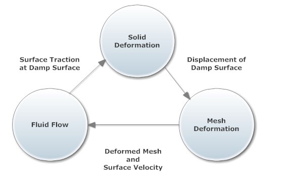
Рисунок 395: Цикл прямого взаимодействия жидкости и конструкции (DC-FSI)

Целевые приложения

Возможность DC-FSI направлена ​​на моделирование податливого структурного реакции на поток жидкости и его сложную взаимосвязь. Эта возможность особенно подходит для задач, демонстрирующих нелинейный структурный отклик. Ее также можно использовать для линейного структурного отклика; однако для линейного структурного отклика решение P-FSI, предлагаемое AcuSolve, может быть более эффективным при решении линеаризованного структурного реакции с нелинейным решением потока. Для получения дополнительной информации о методе P-FSI см. Справочное руководство по командам AcuSolve. Большинство функций PRADIOS, включая нелинейные материалы, нелинейные геометрические эффекты и контакт, доступны для использования. Интерфейсная область может быть смоделирована с использованием сплошных, оболочечных и балочных элементов. Большинство функций в AcuSolve можно использовать в моделировании DC-FSI. Эти функции могут включать, а именно, ламинарный или турбулентный поток, теплопередачу, богатый набор опций материалов, свободную поверхность и многовидовые потоки. Задачи с подвижной границей моделируются с использованием технологий произвольной лагранжево-эйлеровой (ALE) и скользящей сетки. Для получения более подробной информации обратитесь к AcuSolve Справочному руководству по командам.

Основные области применения, на которые рассчитана эта возможность, включают:

• Автомобильная промышленность: резиновые опоры с гидравлическим демпфированием, дверные уплотнители, амортизаторы, конструкция клапанов и резиновых диафрагм, а также антиблокировочные тормозные системы

• Нефть/газ: длинные морские стояки, швартовы, свободные пролеты и буровые стояки

• Авиация и космонавтика: упругость крыла, беспилотные летательные аппараты и беспилотные летательные аппараты

• Ветряные турбины: большая деформация лопастей

• Потребительские товары: дизайн и упаковка

• Биомедицина

см так же

Взаимодействие жидкости и конструкции

DC-FSI с использованием PRADIOS и AcuSolve

Следующий рабочий процесс настоятельно рекомендуется для решения задач DC-FSI:

1. Разработать структурную модель PRADIOS и модель жидкости только для AcuSolve и убедиться, что несвязанные анализы выполняются успешно.

2. Подготовить автономные модели, включающие команды DC-FSI.

3. Запустить связанный анализ.

4. Постобработать решение FSI.

Этот рабочий процесс гарантирует, что модели PRADIOS и AcuSolve определены правильно перед выполнением сопряженного моделирования. PRADIOS и AcuSolve не требуют, чтобы анализ выполнялся с определенной системой единиц, но оба анализа должны использовать согласованную систему единиц. Как правило, все величины, которыми обмениваются два решателя, будут в размерной форме, а компоненты всех векторных величин будут разрешены в инерциальной системе отсчета. Для согласованности для PRADIOS и AcuSolve должны быть выбраны идентичные инерциальные системы отсчета.

Модель PRADIOS

Подготовка модели PRADIOS для DC-FSI включает три шага:

1. Создать входную колоду для PRADIOS

2. Определить область интерфейса и объемы обмена решениями

3. Определить схему связи

Входные данные PRADIOS FSI, имеющие ключевое слово Engine /IMPL/DYNA/FSI is:

/IMPL/DYNA/FSI
ESET SSET PORT MINX MAXX TAG DATA MSG WAIT INIT
FTOL DTOL TTOL XTOL

Каждый из элементов данных обсуждается ниже в соответствующей теме.

Влажные поверхности

Влажная поверхность структурной сетки должна быть указана во входных данных PRADIOS FSI. Влажная поверхность может быть указана либо группой элементов, либо поверхностью. Обратите внимание, что структурная сетка на влажной поверхности не обязательно должна соответствовать сетке сопряженной жидкости. AcuSolve будет внутренне проецировать тяги CFD из сетки интерфейса жидкости на несоответствующую структурную сетку влажной поверхности. Отображение узловых сил также поддерживается для структурных элементов балки. Например, стержень, труба или лопасть могут быть смоделированы с помощью простых элементов балки в структурной сетке. Соответствующая сетка жидкости будет содержать фактическую трехмерную геометрию этих элементов балки.

Если влажная поверхность указана группой элементов (ESET), используйте данные /GRBEAM/BEAM/, /GRSHEL/SHEL/ или /GRSH3N/SH3N/ для балочных, 4-узловых и 3-узловых оболочечных элементов соответственно. Можно указать влажную поверхность твердого тела, покрыв ее оболочечными элементами, а затем присвоить этим элементам нулевые свойства материала с помощью данных /MAT/LAW0. Если влажная поверхность состоит из балочных элементов, то их необходимо указать с помощью данных группы балочных элементов. Идентификатор группы элементов является первым элементом данных /IMPL/DYNA/FSI.

Влажная поверхность (SSET) также может быть указана данными PRADIOS``/SURF``. Данные /SURF имеют множество параметров, которые можно использовать для указания поверхности. Поверхность может быть либо поверхностью оболочечной структуры, либо поверхностью сплошной сетки. Идентификатор поверхности является вторым элементом /IMPL/DYNA/FSI данных. Элементы балки не могут быть указаны с использованием данных /SURF.

Примечание: Влажная поверхность может быть определена комбинацией группы элементов и поверхности.

Соответствующая поверхность жидкости указывается в данных AcuSolve с помощью команды EXTERNAL_CODE_SURFACE.

В некоторых случаях часть структурной влажной поверхности должна быть «помечена», чтобы AcuSolve могла связать ее с граничной поверхностью AcuSolve. Это делается путем указания идентификатора детали PRADIOS в качестве параметра external_code_tags` в данных EXTERNAL_CODE_SURFACE.

Пример:

EXTERNAL_CODE_SURFACE( "Drill" ) {
     ...
        external_code_tags = {"10"}
        ...
}

Данные используются для указания того, что эта поверхность соответствует детали PRADIOS с идентификатором 10. Обратите внимание, что каждая отдельная поверхность должна состоять из элементов с одинаковым идентификатором детали, а каждая отдельная поверхность должна состоять из элементов с отдельными идентификаторами детали. Чтобы применить тег, поверхность твердой структуры, твердое тело должно быть покрыто элементами оболочки, а идентификатор свойства этих элементов оболочки должен использоваться в качестве тега поверхности. Чтобы указать использование тегов поверхности, установите элемент 10 данных /IMPL/DYNA/FSI (TAG) на 1.

Модель AcuSolve

В этом разделе представлен обзор подготовки модели AcuSolve для DC-FSI. Подробную информацию о командах см. в Справочном руководстве по командам AcuSolve. Три шага для подготовки модели AcuSolve:

1. Установите параметры анализа для включения внешнего поля.

2. Определите стратегию решения.

3. Определите определение внешней поверхности.

Настройка параметров анализа для включения внешнего поля

Используйте команду EQUATION для указания доступных полей решения или системы уравнений, которые присутствуют в задаче. Чтобы включить поле, вычисляемое с помощью внешнего решателя, для PRADIOS установите external_codeparameter на ‘ON’.

Например, при проведении анализа структуры жидкости, в котором AcuSolve вычисляет поток, а PRADIOS вычисляет смещения, включите параметр external_code и разрешите произвольное движение сетки, установив параметр mesh на arbitrary_lagrange_eulerian.

EQUATION {
flow = navier_stokes
mesh = arbitrary_lagrange_eulerian
external_code = on
}

Определить стратегию решения

В сочетании с командой EQUATION, которая указывает на наличие полей решения в задаче, необходимо использовать команды TIME_SEQUENCE и STAGGER для определения стратегии пошагового и ступенчатого перемещения по времени. Предпочтительным методом является использование команды AUTO_SOLUTION_STRATEGY, чтобы AcuSolve сгенерировал команды стратегии решения. Чтобы выделить команды стратегии решения, выделите команды TIME_SEQUENCE и STAGGER.

Команда TIME_SEQUENCE указывает стратегию пошагового и ступенчатого перемещения по времени.

В следующем примере сначала решается внешнее поле

для структурных смещений, за которым следует смещение сетки (ALE), в котором корректируются элементы жидкости. Затем решаются уравнения потока и турбулентности.

TIME_SEQUENCE {
 min_time_steps = 1
 max_time_steps = 15
:
 min_stagger_iterations = 1
 max_stagger_iterations = 20
 staggers = { "external_code",
 "mesh_displacement",
 "flow",
 "turbulence" }

}

Для каждого из решаемых полей (каждый шаг, определенный в команде TIME_SEQUENCE) необходимо определить нелинейную итерацию и линейные параметры решателя с помощью команды STAGGER. Например, команды STAGGER показаны для уравнений external_code, mesh_displacement и flow.

 STAGGER ( "external_code” ) {
  уравнение = внешний_код
 min_stagger_iterations = 1
 max_stagger_iterations = 10
                            }
 STAGGER( "mesh_displacement" ) {
 уравнение = mesh_displacement
  min_stagger_iterations = 1
  max_stagger_iterations = 5
  convergence_tolerance = 0.1
  linear_solver = conjugate_gradient
  min_linear_solver_iterations = 10
  max_linear_solver_iterations = 1000
  linear_solver_tolerance = 0.001
  проекция = выкл
  }
STAGGER( "поток" ) {
  уравнение = поток
  min_stagger_iterations = 1
  max_stagger_iterations = 2
  converence_tolerance = 0,1
  lhs_update_frequency = 1
  linear_solver = gmres
  linear_solver_tolerance = 0,1
}

Определение интерфейса жидкость-конструкция

Используйте команду EXTERNAL_CODE_SURFACE для определения интерфейса между жидкостью и конструкцией. Команда определяет топологию поверхности, а также свойства интерфейса.

В следующем примере топология поверхности интерфейса считывается из файла wall.ebc, расположенного в каталоге MESH.DIR, и состоит из 3-узловых треугольников. velocity_type, temperature_type и mesh_displacement_type определяют свойства интерфейса (граничные условия) и являются:

EXTERNAL_CODE_SURFACE( "wall" ) {
  surfaces = Read( "MESH.DIR/wall.ebc" )
  shape          = "three_node_triangle"
  element_set = "tet fluid"
  velocity_type = wall
  temperature_type = tied
  mesh_displacement_type = tied
  gap = 0
  gap_factor = 0
  external_code_tags = {}
}

Свойства интерфейса или граничные условия задаются с помощью параметров mesh_displacement_type, velocity_type и temperature_type. Параметр mesh_displacement определяет, будет ли сетка жидкости привязана к твердотельной сетке или ей разрешено скользить по твердотельной поверхности сетки. Установите mesh_displacement_type=tied, чтобы связать сетку жидкости с твердой сеткой, или mesh_displacement_type=slip, чтобы позволить сетке жидкости скользить по твердой поверхности, которая действует как направляющая поверхность.

velocity_type определяет, как скорость жидкости ведет себя по отношению к скорости структурной сетки.

Установите velocity_type=wall, чтобы связать скорость жидкости со скоростью сетки, или установите velocity_type=slip, чтобы нормальная составляющая скорости жидкости была привязана к скорости твердотельной сетки.

Существует четыре возможных комбинации интерфейсов, основанных на настройках параметров mesh_displacement и velocity_type. Они обобщены в Таблице 23.

Таблица 23: Граничные условия прямого взаимодействия жидкости и конструкции

Жидкость-Твердое **Интерфейс Условия **		Смещение сетки
		Связан	Проскальзывание
Тип скорости	Стена	\(x_{fluid}=x_{ solid}\) \(u_{fluid}=\big{(} x_{fluid}^{n+1}-x_{fluid} ^{n}\big{)}/\Delta t\)	\(x_{fluid}\in S_{ solid}\) \(u_{fluid}=\cdot n=\big{(}x_{fluid}^{n+1} -x_{fluid}^{n}\big{)} /\Delta t\cdot n\) \(u_{fluid}\cdot t_ {i}=\big{(}x_{fluid}^ {n+1}-x_{solid}^{n} \big{)}/\Delta t\cdot t _{i}i=1,2\)
	Соскаль- зывать	\(x_{fluid}=x_{ solid}\) \(u_{fluid}\cdot n= \big{(}x_{fluid}^{n+1}- x_{fluid}^{n}\big{)}/ \Delta t\cdot n\)	\(x_{fluid}\in S_{ solid}\) \(u_{fluid}=\cdot n=\big{(}x_{fluid}^{n+1} -x_{fluid}^{n}\big{)}/ \Delta t\cdot n\)

Когда жидкость может скользить по твердой сетке, поиски окрестностей между

жидкой и твердой сетками выполняются непрерывно.

Параметр gap_factor указывает безразмерный (по отношению к длине грани элемента) максимально допустимый зазор, а параметр gap указывает размерное максимальное расстояние зазора между каждой квадратурной точкой поверхности AcuSolve до ближайшей

поверхности, заданной PRADIOS для проверки зазоров. Если расстояние больше зазора,

вычисление останавливается с сообщением об ошибке.

Связь между PRADIOS и AcuSolve

PRADIOS и AcuSolve могут работать на гетерогенных и удаленных платформах, расположенных в одном сетевом домене. Связь между PRADIOS и AcuSolve осуществляется через сокеты. Чтобы начать совместное моделирование между PRADIOS и AcuSolve, одно из аналитических программ должно инициировать процесс связи, в то время как другое аналитическое программное обеспечение должно подключиться к инициированному процессу связи.

В PRADIOS номер порта сокета (PORT) указывается третьим элементом данных /IMPL/DYNA/FSI. Номер порта по умолчанию - 10000. Этот же номер порта должен быть указан в данных EXTERNAL_CODE в файле AcuSolve.inp. Если машина, на которой запущен PRADIOS, называется linux_mach, то EXTERNAL_CODE будет выглядеть так:

EXTERNAL_CODE {
communication = socket
socket_initiate = no
socket_host = "linux_mach"
socket_port = 10000
}

AcuSolve и PRADIOS запускаются независимо. AcuSolve будет ждать, пока PRADIOS инициирует сокетное соединение. Время, которое AcuSolve будет ждать, определяется параметром WAIT данных /IMPL/DYNA/FSI. Значение по умолчанию составляет 3600 секунд.

Перед началом цикла временного шага необходимо обменять базовую информацию об интерфейсе между двумя кодами. Во-первых, для обоих кодов необходимо задать ряд параметров, управляющих стратегией интерфейса. Во-вторых, необходимо определить физические параметры интерфейса. Обычно и AcuSolve, и PRADIOS запускаются на одном и том же временном шаге; Однако, если есть желание, чтобы AcuSolve запустился первым (чтобы поток мог развиваться), данные INIT данных /IMPL/DYNA/FSI можно установить на начальный временной шаг AcuSolve, с которого начнется связанный анализ.

Временные шаги и обмен данными

Оба PRADIOS и AcuSolve должны использовать один и тот же размер временного шага, а общее количество временных шагов должно быть одинаковым. Кроме того, размер временного шага должен оставаться постоянным как в PRADIOS, так и в AcuSolve. Например, для 1000 временных шагов 0,001 секунды данные AcuSolve и PRADIOS являются:

AUTO_SOLUTION_STRATEGY { initial_time_increment = 0.001 max_time_steps = 1000 min_stagger_iterations = 1 max_stagger_iterations = 20 }

и

/RUN/wing/1
1.0
/IMPL/DTINI
0.001
/IMPL/DT/2
        12  0.0  120  1.0  1.0

Для входных данных PRADIOS /IMPL/DT/2 пункты 4 и 5 определяют масштабные коэффициенты шага по времени. Их необходимо установить на 1,0, чтобы сохранить постоянный шаг по времени PRADIOS.

На каждом шаге по времени силы и смещения обмениваются между PRADIOS и AcuSolve, пока они не сойдутся до определенного допуска. После достижения сходимости анализ продолжается на следующем шаге по времени. Эти обмены называются «стаггерами» в AcuSolve. Минимальное количество стаггеров (обменов) должно быть установлено на 1 в обоих наборах входных данных. Это указывается параметром min_stagger_iterations в данных AcuSolve AUTO_SOLUTION_STRATEGY и данными MINX в данных PRADIOS /IMPL/DYNA/FSI.

Максимальное количество обменов можно контролировать с помощью комбинации критериев сходимости силы и смещения и жесткого ограничения максимального количества обменов. Максимальное количество обменов задается параметром max_stagger_iterations в данных AcuSolve AUTO_SOLUTION_STRATEGY и данными MAXX в данных PRADIOS /IMPL/DYNA/FSI.

Допуски сходимости силы и смещения используются для сокращения количества обменов до числа, необходимого для получения стабильных и точных результатов. Это может значительно сократить время выполнения, гарантируя точные результаты. Допуски силы и смещения указаны данными FTOL и DTOL в данных PRADIOS /IMPL/DYNA/FSI. Это допуски на нормы L2 векторов силы и смещения. Если эти допуски установлены высокими, время решения будет сокращено, но точность решения также может быть снижена.

Обычно необходимо обмениваться только силами и смещениями. В особых случаях, таких как вращающаяся балка, вы можете запросить, чтобы также обменивались моменты и вращения. Это делается путем установки параметра DATA на 2 в данных PRADIOS /IMPL/DYNA/FSI.

Проверка обмена данными

Чтобы проверить, что обмен данными между PRADIOS и AcuSolve происходит правильно, параметр MSG может быть установлен на ненулевое значение данных PRADIOS /IMPL/DYNA/FSI. Чем выше значение, тем больше объем информации, которая записывается в файл PRADIOS .out для проверки. Эти данные включают в себя параметры управления передачей данных, а также фактические значения сил и моментов, которыми обмениваются.

Примеры

Обычно вам нужно только определить влажную поверхность для запуска Анализа взаимодействия жидкости и конструкции с PRADIOS и AcuSolve. Если влажная поверхность имеет идентификатор поверхности 10, входные данные будут:

/IMPL/DYNA/FSI
0 10 0 0 0 0 0 0 0 0
0 0 0 0

В этом случае все остальные параметры FSI устанавливаются на свои значения по умолчанию. В PRADIOS 0 означает значение по умолчанию, а не явно ноль (если только значение по умолчанию на самом деле не равно нулю).

Чтобы сократить время выполнения, вы можете установить верхнюю границу для количества обменов, а также установить более высокие значения для допусков сходимости силы и смещения. Например, вы можете установить максимальное количество обменов на 5, а допуски сходимости силы и смещения на 0,01 и 0,005 соответственно с данными FSI:

/IMPL/DYNA/FSI
0 10 0 0 5 0 0 0 0
0 0.01 0.005 0 0

В случае балочной задачи с маркированными элементами и обменом моментами и вращениями входные данные будут следующими:

/IMPL/DYNA/FSI 20 0 0 0 0 1 1 0 0 00 0 0 0

Где 20 — это набор элементов, содержащий все элементы балки. Теги элементов балки основаны на идентификаторах свойств балки.

Настройка данных PRADIOS Structural FSI

Тип структурного анализа — неявная динамика, и он решается с использованием Общего метода Ньюмарка, поэтому ключевое слово PRADIOS Engine:

/IMPL/DYNA/2

Предлагаемые критерии сходимости шага времени PRADIOS составляют 0,001 для энергии и силы и 0,01 для смещения, как установлено в неявных нелинейных данных управления решением:

/IMPL/NONLIN/1
123 0.001 0.001 0.01

Поскольку временной шаг должен оставаться постоянным, метод управления временным шагом должен допускать множество временных итераций без изменения временного шага, а масштабные коэффициенты на временном шаге должны быть 1.0. Данные метода управления временным шагом 2 должны быть:

/IMPL/DT/2
12 0.0 120 1.0 1.0

Также, количество допустимых итераций расхождения должно быть увеличено, чтобы не корректировать временной шаг. Это делается путем установки критерия расхождения на 5 с:

/IMPL/DIVERG/5

Наконец, чтобы записать приложенные нагрузки от тяги жидкости и результирующие смещения в файлы анимации PRADIOSresults, используйте:

/ANIM/VECT/FEXT
/ANIM/VECT/DISP

Расположение моделей

Модели PRADIOS и AcuSolve должны быть совмещены. Другими словами, сетка границы жидкости и соответствующая структурная сетка влажной поверхности соответствуют друг другу как физическая граница. Зазор между этими сетками должен быть небольшим. Чтобы проверить соответствие поверхностей обмена в AcuSolve, обратитесь к файлу .Log для получения информации о структурной сетке, как показано ниже. Проверьте количество элементов влажной поверхности и минимальные и максимальные координаты влажной поверхности, а также для соответствия ограничивающей рамки и областей, чтобы помочь определить положение, размер и ориентацию несоответствие:

acuSolve: Количество внешних узлов кода = 15050
acuSolve: Количество внешних узлов кода tri3s = 0
acuSolve: Количество внешних узлов кода quad4s = 15000
acuSolve: Мин/Макс x-координата = -3,812500e-02 3,812500e-02
acuSolve: Мин/Макс y-координата = -3,805000e-02 3,805000e-02
acuSolve: Мин/Макс z-координата = 0,000000e+00 3,812500e+00
acuSolve: Общая площадь поверхности = 9,126732e-01
acuSolve: Количество поверхностей с жидкой влажностью = 5637
acuSolve: Мин/Макс x-координата = -3.812499e-02 3.812500e-02
acuSolve: Мин/Макс y-координата = -3.812494e-02 3.812498e-02
acuSolve: Мин/Макс z-координата = 0.000000e+00 3.812500e+00
acuSolve: Общая площадь поверхности жидкости = 9.128247e-01

На каждом временном шаге влажная поверхность деформируется из-за нагрузки потока жидкости. В то же время сетка жидкости перемещается, чтобы соответствовать новой влажной поверхности. Средний и максимальный зазор между сетками показан для каждого временного шага как:

acuSolve: Среднее расстояние = 2,842759e-05
acuSolve: Макс. расстояние = 1,182390e-04

Разрыв должен оставаться небольшим для допустимого решения.

Постобработка связанного моделирования

Есть несколько вариантов постобработки связанного моделирования:

• Постобработка структурного решения и реакции интерфейса с помощью HyperView, а также жидкостного решения и реакции интерфейса с помощью постпроцессора, совместимого с AcuSolve, например HyperView.

• Используйте стороннее программное обеспечение для постобработки для постобработки объединенного структурного и жидкостного решения.

Масштабирование величин

Вы можете применить функцию множителя в AcuSolve к силам и/или моментам, импортированным из PRADIOS. Поля масштабирования могут быть полезны при запуске моделирования взаимодействия жидкости и конструкции с высокими инерционными эффектами. Укажите функцию множителя в команде EXTERNAL_CODE.

MULTIPLIER_FUNCTION("ramp" ) {
type = piecewise_linear
curve_fit_values = { 1, 0.0 ; 10 , 1 }
curve_fit_variable = time_step
  }
     EXTERNAL_CODE {
     …
multiplier_function = "ramp"
…
  }

Параллельное выполнение решателей

AcuSolve и PRADIOS могут работать параллельно на распределенных кластерах памяти.

Поддержка платформ

AcuSolve работает на Windows (64-разрядной) и Linux (64-разрядной).

Ограничения

• Если влажная поверхность содержит балочные элементы, никакие другие элементы не могут быть использованы для определения влажной поверхности. Другими словами, балочные элементы не могут быть смешаны с другими элементами для определения влажной поверхности.

• Квадратичные и модифицированные тетраэдральные элементы не поддерживаются

• Между двумя решателями должно быть постоянное фиксированное приращение шага времени

• Термический анализ в настоящее время не поддерживается

Примечания к квазистатическому анализу

При выполнении квазистатического анализа (/IMPL/QSTAT) положительно определенное свойство матрицы жесткости будет усилено включением матрицы инерции. Дополнительная жесткость является функцией масс, инерции и шага по времени. Меньшие шаги по времени добавят больше жесткости. Кроме того, для добавленной матрицы можно определить масштабный коэффициент с помощью ключевого слова /IMPL/QSTAT/DTSCAL (этот коэффициент обратно пропорционален этой добавленной матрице, как и шаг по времени). Для нелинейного анализа это изменит только скорость сходимости; тогда как для линейного анализа шаг по времени (один шаг) следует выбирать осторожно (не слишком мал, так как это значительно изменит результат; и не слишком велик, так как это может привести к неположительно определенной матрице).

Этот вариант вполне подходит для модели, которая состоит из частей, соединенных только контактными интерфейсами, и не прошла другие типы анализа. Линейный квазистатический анализ также может использоваться для проверки модели высокого уровня (даже для явного анализа). При использовании не слишком большого временного шага результаты всегда могут быть получены, независимо от того, хорошо ли ограничена модель или нет.

Как упоминалось в Активации неявного анализа, когда /IMPL/QSTAT/DTSCAL используется с /IMPL/LINEAR/INTER (два шага), коэффициент масштабирования применяется только на втором шаге. Тщательно выбрав этот коэффициент масштабирования и время завершения, можно найти правильный контакт на первом шаге и минимизировать ошибку (из-за дополнительной жесткости) на последнем шаге.

Типичным примером этой методологии является моделирование начального состояния под действием силы тяжести полного автомобиля с манекенами, в котором манекены связывают автомобиль только посредством контакта. Определяется короткое время остановки, так что большого смещения между частями не происходит во время исследования контакта на первом шаге, а большой

квазистатический коэффициент масштабирования применяется для второго шага, чтобы получить статическое решение.

Заметки о нелинейном неявном анализе

В нелинейном неявном анализе, когда формулировки элементов различаются между построением матрицы жесткости и расчетом внутренней силы (так же, как и явная), часто наблюдаются проблемы со сходимостью; это особенно верно для элементов сокращенной интеграции с управлением возмущением песочных часов. С другой стороны, можно получить сходимые результаты с элементами похожих формулировок, такими как QEPH и QBAT для оболочек или HA8, HC8, S8 и HEPH для твердых тел. В любом случае предпочтительны те же формулировки.

Как упоминалось ранее, PRADIOS использует только упругую часть параметров материала для построения матрицы жесткости, что позволяет работать со всеми доступными материалами PRADIOS. Еще одним преимуществом использования упругой матрицы жесткости является то, что проблемы со сходимостью избегаются с определенными материалами (например, упругопластическими). Некоторые примеры тестов показали, что упругая матрица жесткости, связанная с линейным поиском, обеспечивает разумную сходимость для нелинейных материальных расчетов. Конечно, метод Ньютона-Рафсона (с использованием касательной матрицы) также может быть добавлен в будущем. Единственное исключение из использования упругой части материала — это случай пружинных элементов, которые не связаны с какими-либо материальными законами. Когда нелинейная функция определена в свойстве пружины для неявного нелинейного анализа, будет вычислена элементарная матрица касательной жесткости. Однако, чтобы избежать проблем со сходимостью в нелинейном анализе, матрица упругой жесткости по-прежнему используется для упругопластических пружин (H>0). В линейном анализе с пружинными элементами, если были определены нелинейные функции жесткости, линейная жесткость вычисляется, используя только первые точки (кроме 0, 0) этой функции.

Проблемы со сходимостью часто встречаются в нелинейном анализе, в котором управляющие параметры играют важную роль. Эти параметры зависят от задачи, и входные значения могут определять сходимость или неудачу вычисления. Лучшие значения часто являются хорошим компромиссом между качеством и производительностью.

Сначала необходимо ввести параметры управления для нелинейного решателя.

Формат этого ключевого слова:

/IMPL/NONLIN/n
L_A Itol Tol

Доступны два нелинейных решателя: - Модифицированный метод Ньютона (n=1)

• Метод Квази-Ньютона (BFGS) (n=2)

  L_A

  Этот параметр задает максимальное количество итераций для реформирования матрицы жесткости; рекомендуется значение 3 для итеративного решателя и значение 6 для прямого или смешанного решателя.

  Itol

  Критерии, используемые для прекращения выполнения.

  1. Относительный остаток в энергии

  2. Относительный остаток в силе

  Tol

  Значение допуска; итерация считается сходящейся, если относительное остаточное значение (остаточное значение по сравнению с опорным значением) равно или меньше допуска.

Опорные значения вычисляются при нулевой итерации (выходные сообщения).

В PRADIOS обновленная матрица жесткости имеет смысл в основном в геометрии (используя упругий параметр для нелинейных материалов); поэтому небольшое значение для L_A обеспечит более быструю сходимость, в зависимости от уровня приращения смещения, но с большими затратами на вычисления для реформирования матрицы жесткости; это особенно верно для прямого решателя.

Обычно критерий остановки по силе (Itol =2) обеспечивает лучший результат по балансу,

что является критерием по умолчанию. Критерий по энергии может

легко сходиться и лучше подходит для моделирования упруго-пластичных материалов при монотонно возрастающей нагрузке; поскольку в этом случае энергия увеличивается сильнее, чем сила (которая вырабатывается пластическими допустимыми напряжениями), сходимость становится легче из-за тех же самых изменений опорных значений (чем выше опорное значение, тем легче сходимость).

Во-вторых, следует выбирать управление временным шагом при использовании ключевых слов /IMPL/DT/n и /IMPL/DTINI. Если метод управления временным шагом не определен, во время нелинейного моделирования используется постоянный временной шаг (не рекомендуется). Для более эффективного управления временным шагом доступны два метода автоматического управления временным шагом (n=1 или 2). Первый метод — это метод линейного поиска, который работает только в соответствии с сошлисьми числами итераций. Второй метод — это метод управления смещением, подобный длине дуги, и рекомендуется для общего использования.

Когда на каждом шаге (цикле) используется автоматическое управление временным шагом, решатель PRADIOS автоматически корректирует временной шаг с входными масштабными коэффициентами. Если итерация расходится, PRADIOS уменьшит масштаб временного шага, а затем перезапустит итерацию.

Коэффициенты масштабирования по умолчанию — 0,67 (для уменьшающегося коэффициента) и 1,1 (для максимального увеличения, то есть максимального коэффициента, на который будет увеличен временной шаг).

Использование максимального увеличивающегося коэффициента, ближе к единице, например: 1,01, обеспечит более легкую сходимость для сложных анализов, таких как выпучивание.

Также следует определить начальный временной шаг с помощью ключевого слова /IMPL/DTINI. Это дает приблизительное количество шагов, необходимых для моделирования.

Для запуска нелинейного моделирования может потребоваться достаточное количество шагов (обычно > 100), поскольку:

1. Модели с геометрической или контактной нелинейностью сходятся легче с малыми шагами.

2. Некоторое поведение материалов, особенно зависящее от пути, требует малых шагов для точной интеграции.

Также очень полезно установить пределы Min и Max для временного шага, используя``/IMPL/DT/STOP``.

DT_min

Для остановки вычислений в случае расхождения.

DT_max

Устанавливает потолок для временного шага. Вычисления не остановятся при достижении этого значения; но это полезно для сходимости высоконелинейных симуляций или просто для выходных потребностей.

Перезапуск PRADIOS также доступен с неявным анализом. В этом случае можно определить различные параметры для сходящихся стратегий.

Нелинейный анализ с контактом

Относительная остаточная сила (по умолчанию) рекомендуется для нелинейного анализа с контактом.

Как и в явном анализе, больший зазор для контактов приводит к лучшей сходимости. Это особенно верно для интерфейса TYPE 11, где необходимо установить достаточное значение зазора, чтобы избежать прекращения вычислений из-за уменьшения шага по времени. Для моделирования с контактом (например: начальное состояние штамповки под действием силы тяжести, детали, ограниченные контактами) с использованием интерфейса TYPE 7 с небольшим начальным зазором, определение \(Gap_{min}\) немного большего, чем начальный зазор, приведет к лучшей сходимости. Начальные проникновения будут быстро восстанавливаться.

Если контакт определен с трением, то рекомендуется формулировка инкрементальной жесткости (\(I_{form} =2\)).

Поскольку сложно выбрать подходящее опорное значение в анализах с контактами (особенно при моделировании, включающем жесткие детали с наложенным смещением, воздействующим на деформируемую часть), PRADIOS делает исключение, изменяя опорное значение в первой итерации. Если относительная невязка становится слишком большой (>>1), PRADIOS перезапустит итерацию с меньшим шагом по времени и более высоким опорным значением. Измененное опорное значение иногда является произвольным и слишком высоким, поэтому вы должны проверить это значение (распечатку на нулевой итерации на каждом шаге), так как это может привести к сходимости с неправильным результатом. Это также может быть верно, когда в определении интерфейса присутствуют высокие начальные проникновения.

При использовании интерфейса TYPE 7 контактная жесткость играет важную роль в сходимости,

поэтому рекомендуется \(I_{stf}\) = 4 (что принимает минимум

основной и вторичной жесткости для контакта). Это связано с причиной, указанной в предыдущем абзаце, а также с тем, что штрафная контактная сила будет уравновешена внутренней силой деформируемой ударной части. Это означает, что жесткость, близкая к эффективной жесткости, будет сходиться легче, чем более высокая. Иногда жесткость с уменьшением масштабного коэффициента (например: Stfac 0,01) или уменьшением толщины ударника (если он жесткий) может уменьшить несбалансированные силы и улучшить сходимость, особенно в оболочечных конструкциях при изгибе, где эффективная жесткость намного ниже мембранной жесткости; но следует отметить, что слишком низкое значение также может привести к расхождению.

Анализ взаимодействия жидкости и конструкции с помощью PRADIOS и AcuSolve

Примечание: Поддержка прямого сопряженного взаимодействия Fluid-Structure (DC-FSI) PRADIOS и AcuSolve прекращена. Теперь рекомендуется использовать OptiStruct в сочетании с AcuSolve, как описано в разделе «Взаимодействие Fluid-Structure» в Руководстве пользователя OptiStruct.

PRADIOS и AcuSolve полностью интегрированы для выполнения анализа прямого сопряженного взаимодействия жидкости и конструкции (DCFSI) на основе разделенного ступенчатым подходом. PRADIOS и AcuSolve являются кодами моделирования во временной области, которые разбивают сопряженное моделирование на ряд временных шагов. Поскольку основные уравнения PRADIOS и AcuSolve являются нелинейными, обычно требуются субитерации на каждом временном шаге. На каждой субитерации анализа FSI тяги жидкости в AcuSolve преобразуются в узловые силы, которые затем переносятся в структурную интерфейсную сетку PRADIOS. Эти силы используются для расчета деформации конструкции с использованием PRADIOS. Обратите внимание, что в дополнение

к

нагрузке от тяг потоков жидкости могут также применяться дополнительные структурные нагрузки. Полученная деформированная форма конструкции передается обратно в AcuSolve в качестве новой границы жидкости. Этот цикл FSI показан ниже на рисунке 396.

Рисунок 396: Цикл прямого взаимодействия жидкости и конструкции (DC-FSI)

Целевые приложения

Возможность DC-FSI направлена ​​на моделирование податливого структурного реакции на поток жидкости и его сложную взаимосвязь. Эта возможность особенно подходит для задач, демонстрирующих нелинейный структурный отклик. Ее также можно использовать для линейного структурного отклика; однако для линейного структурного отклика решение P-FSI, предлагаемое AcuSolve, может быть более эффективным при решении линеаризованного структурного реакции с нелинейным решением потока. Для получения дополнительной информации о методе P-FSI см. Справочное руководство по командам AcuSolve. Большинство функций PRADIOS, включая нелинейные материалы, нелинейные геометрические эффекты и контакт, доступны для использования. Интерфейсная область может быть смоделирована с использованием сплошных, оболочечных и балочных элементов. Большинство функций в AcuSolve можно использовать в моделировании DC-FSI. Эти функции могут включать, а именно, ламинарный или турбулентный поток, теплопередачу, богатый набор опций материалов, свободную поверхность и многовидовые потоки. Задачи с подвижной границей моделируются с использованием технологий произвольной лагранжево-эйлеровой (ALE) и скользящей сетки. Для получения более подробной информации обратитесь к AcuSolve Справочному руководству по командам.

Основные области применения, на которые рассчитана эта возможность, включают:

• Автомобильная промышленность: резиновые опоры с гидравлическим демпфированием, дверные уплотнители, амортизаторы, конструкция клапанов и резиновых диафрагм, а также антиблокировочные тормозные системы

• Нефть/газ: длинные морские стояки, швартовы, свободные пролеты и буровые стояки

• Аэрокосмическая промышленность: упругость крыла, беспилотные летательные аппараты и беспилотные летательные аппараты

• Ветряные турбины: большая деформация лопастей

• Потребительские товары: проектирование и упаковка

• Биомедицина

См. также

Интеграция жидкости и конструкции

Выходные сообщения

Ниже приведена часть распечатки (на шаге 2 выходного файла Engine _0001.out), когда в файле Engine (_0001.rad) используется ключевое слово /IMPL/PRINT/NONLIN/n):

ВРЕМЯ ЦИКЛА ВРЕМЯ-ШАГ ЭЛЕМЕНТ ОШИБКА I-ЭНЕРГИЯ K-ЭНЕРГИЯ T K-ЭНЕРГИЯ R EXT-W
-------
 2 2.380    0.4802   SHELL    0.0%  5.117    0.000    0.000    5.117
   --СОЗДАНА ДОПОЛНИТЕЛЬНАЯ МАТРИЦА ЖЕСТКОСТИ КОНТАКТА--
     С РАЗМЕРАМИ: ND = 141 NZ = 1050 NB_MAX = 15
     NL_ITERATION= 0 НАЧАЛЬНАЯ ОСТАТОЧНАЯ НОРМА= 0.5913E+01 0.4613E+04 0.1600E+05
  --МАТРИЦА ЖЕСТКОСТИ ПРЕОБРАЗОВАНА --
  --СОЗДАНА ДОПОЛНИТЕЛЬНАЯ МАТРИЦА ЖЕСТКОСТИ КОНТАКТА--
    С РАЗМЕРАМИ: ND = 141 NZ = 1050 NB_MAX = 15
    NL_ITERATION= 0 НАЧАЛЬНАЯ ОСТАТОЧНАЯ НОРМА= 0.5913E+01 0.4613E+04 0.1600E+05
  --МАТРИЦА ЖЕСТКОСТИ ПРЕОБРАЗОВАНА --
  --МАТРИЦА ЖЕСТКОСТИ КОНТАКТА--
  С РАЗМЕРАМИ: : ND = 150 NZ = 1059 NB_MAX = 15
  NL_ITERATION= 1 ОТНОСИТЕЛЬНАЯ НОРМА ОСТАТКА= 0,1000E+01 0,8593E-01 0,5005E-01
  --СОЗДАНА ДОПОЛНИТЕЛЬНАЯ МАТРИЦА ЖЕСТКОСТИ КОНТАКТА--
  С РАЗМЕРАМИ: ND = 156 NZ = 1101 NB_MAX = 15
  СХОДИТСЯ С 2 ИТЕРАЦИЯМИ, |du|/|u|,|r|/|r0|,|dE|/|E|= 0.5915 0.4747E-01 0.1166

Каждая итерация содержит распечатку нормализованных (норма L2) начальных значений (итерация ноль) или относительных значений смещения, остаточной силы и энергии. Таким образом, |du|/|u| — относительная остаточная величина смещения, |r|/ |r0| — относительная остаточная величина силы, а |dE|/|E| — относительная остаточная величина энергии.

Настройка матрицы жесткости

В начале каждого вычисления выводится следующее сообщение:

*--------- НАСТРОЙКА МАТРИЦЫ ЖЕСТКОСТИ ---------*
СИМВОЛИЧЕСКИЙ РАЗМЕР: ND = 164202 NZ = 6047160 NB_MAX = 96
КОНЕЧНЫЙ РАЗМЕР: ND = 154605 NZ = 5652417 NB_MAX = 96

Где,

ND

Размерность матрицы жесткости (количество степеней свободы)

NZ

Количество ненулевых значений строго треугольной матрицы (из-за симметрии матрицы сохраняются только значения ND+NZ)

NB_MAX

Максимальное количество связанных узлов в модели

PRADIOS устраняет все зависимые узлы (этот процесс называется «конденсацией») перед разрешением, и поэтому измерения SYMBOLIC и FINAL соответствуют измерению матрицы до и после конденсации.

Если контакт учитывается, матрица жесткости штрафной пружины хранится независимо, и информация об этом выводится (если /IMPL/PRINT/NONLIN/n определено) после обнаружения контактов:

--СОЗДАЕТСЯ ДОПОЛНИТЕЛЬНАЯ МАТРИЦА ЖЕСТКОСТИ КОНТАКТА --
C DIM. : ND   =  42 NZ    =  42 NB_MAX =       16

Примечание: Распечатывается только информация о конечной (после конденсации) матрице.

В версии PRADIOS SPMD печатается подматрица основной матрицы жесткости, хранящаяся на каждой машине; а для дополнительной контактной матрицы печатается только общая конечная.

• Информация о ЦП

Если ключевое слово /MON/ON определено во входном файле PRADIOS Engine (_0001.rad), некоторая подробная информация о времени обработки ЦП информация о неявной схеме печатается в файле .out:

#PROC [K]SETUP [M]SETUP IMPL.SOLV IMPL.TOTAL

1 .2484E+01 .1528E+02 .6742E+02 .8520E+02

#PROC CONT.SORT CONT. F ELEMENT MAT KIN.COND. INTEGR. I/O TASK0 ASSEMB. RESOL

1 .0000E+00 .0000E+00 .1875 .3125E-01 .0000 .0000E+00 .2188 .2188 .0000 .8561E+02

ПРОШЕДШЕЕ ВРЕМЯ: 89,32 с

Где,

[K]

Основная матрица жесткости

[M]

Матрица предварительной подготовки (если используется итерационный решатель)

IMPL.SOLV

Для разрешения {x}=[K]-1{b}

Числовые значения представляют время.

Вывод решения для каждой итерации (/IMPL/SOLV и /IMPL/NONLIN/SOLVINFO)

Вывод глобальной информации о решении на каждой итерации решения. Эта команда создает три дополнительных файла:

Filename_implicit.info

Для наибольших остатков (силы и момента), наибольших приращений смещения и вращения и наибольших поправок на каждой итерации и каждом приращении.

Filename_implicit.hist

Содержит все данные для построения графиков в Laduga Simulation.

:Filename_implicit.tpl** Скрипт tpl для построения графиков в Laduga Simulation данных из файла .hist.

Устранение неполадок

Когда PRADIOS останавливается с одним из следующих сообщений об ошибке:

Если выводится это сообщение об ошибке, возможны два случая.

МАТРИЦА ЖЕСТКОСТИ НЕ ОПРЕДЕЛЕНА

1. Матрица жесткости (геометрическая) не определена. Это может произойти, когда некоторые значения степеней свободы в матрице жесткости равны нулю (например: одна из вращательных жесткостей пружины TYPE 8 определена как ноль), или модуль упругости материала слишком мал (часто из-за несоответствий в единицах, используемых в модели).

2. Модель все еще имеет моды жесткого тела даже после применения граничных условий. Это более распространенный источник этой ошибки. Примерами являются две части, которые соединены только контактными интерфейсами, или пружина с 6 степенями свободы, соединенная с твердым элементом с 3 степенями свободы.

Моделирование не удается из-за неявного разрешения (обратная матрица), даже с итеративным (PCG) решателем.

PRADIOS implicit автоматически исправит эти свободные степени свободы в первом случае (см. PRADIOS Engine Input для получения более подробной информации).

Чтобы проверить моды жесткого тела во втором случае, используйте один из следующих методов, запустив:

• Проверка модели (с /IMPL/CHECK в файле Engine Input). Результаты этой проверки будут перечислены в файле *n.out.

• Линейный квазистатический анализ (предпочтительно прямой решатель) с достаточно большим шагом по времени. Свободную часть можно найти, просмотрев файлы анимации.

Некоторые возможные обходные пути для устранения таких режимов жесткого тела:

• Добавление искусственных пружин с (малой жесткостью) для соединения свободных частей.

• Создание небольшого начального проникновения в контактах, если интерфейсы определены между свободными частями.

• Запуск квазистатического анализа.

Сообщение об ошибке ниже появляется, когда в модели не определена нагрузка или когда нагрузка равна нулю на первом этапе нелинейного анализа.

IMPLICIT ОСТАНОВЛЕН ИЗ-ЗА ЗАГРУЗКИ ДАННЫХ

Выполнение завершается следующим сообщением PRADIOS:

**PRADIOS IMPLICIT ОСТАНОВЛЕН ИЗ-ЗА ЗАГРУЗКИ ДАННЫХ**
ISTOP =       0

Вот несколько предлагаемых обходных путей:

1. Проверьте загрузку в модели.

2. Увеличьте начальный временной шаг.

3. Создайте небольшое проникновение контакта в случаях, когда загрузка вызвана контактом.

Если выводится сообщение об ошибке, показанное ниже::

ВРЕМЕННОЙ ШАГ УМЕНЬШЕН ИЗ-ЗА ОТКЛЮЧЕНИЯ

Следующее предупреждение может быть выведено в нелинейных симуляциях с контактом:

**ВРЕМЕННОЙ ШАГ БУДЕТ УМЕНЬШЕН, ЧТОБЫ ИЗБЕЖАТЬ ОТКЛЮЧЕНИЯ В ИНТЕРФЕЙСЕ**: 14

В таком случае PRADIOS попытается перезапустить итерацию с уменьшенным временным шагом, и в конечном итоге запуск может завершиться неудачей, если временной шаг упадет ниже предписанного минимума. Это обычно наблюдается в моделях с интерфейсом ТИПА 11 (контакт край-к-краю) с небольшим зазором.

** ОШИБКА: PRADIOS НЕЯВНЫЙ ОСТАНОВЛЕН ИЗ-ЗА ДАННЫХ МОДЕЛИРОВАНИЯ **

ISTOP = - 1

Это сообщение обычно следует за различными сообщениями об ошибках моделирования: “МАТРИЦА ЖЕСТКОСТИ НЕ ОПРЕДЕЛЕНА”, “...СЛИШКОМ БОЛЬШОЕ ЗНАЧЕНИЕ ЭНЕРГИИ”.

Часто дело было в условиях ограничений или слишком большом временном шаге.

**ОШИБКА: PRADIOS НЕЯВНЫЙ ОСТАНОВЛЕН ИЗ-ЗА ОГРАНИЧЕНИЯ ВРЕМЕННОГО ШАГА**

ISTOP = -2

Когда шаг по времени меньше минимального входного шага (см. /IMPL/DT/STOP), PRADIOОстановите бег с помощью этого сообщения.

Причина обычно в проблеме сходимости (DT_min), если DT_min было уже достаточно мало или нет. Нет общего обходного пути для проблемы сходимости, как описано ниже:

1. Добавление дополнительных распечаток в файлы out (/PRINT/n, например, n=1, /IMPL/PRINT/NONLIN/n, например, n=1) и анализ причины сбоя.

2. Проверьте модель, условия ограничений, материалы, определения контактного интерфейса и т. д.

3. Если сбой произошел из-за нестабильности, попробуйте /IMPL/DT/3 (метод Рикса) для моделирования типа snap-thru или /IMPL/QSTAT для случая общей нестабильности.

4. Переключение других критериев сходимости (см. Itol в /IMPL/NONLIN) или потеря допуска, если это возможно.

5. Попробуйте /IMPL/NONL/SMDISP, чтобы узнать, возникла ли проблема из-за геометрической нелинейности.

IMPLICIT ОСТАНОВЛЕН ИЗ-ЗА ОШИБКИ РЕШАТЕЛЯ

Выполнение завершается следующим сообщением PRADIOS:

"**ERROR: PRADIOS IMPLICIT ОСТАНОВЛЕН ИЗ-ЗА ОШИБКИ РЕШАТЕЛЯ**
ISTOP = -4"

Два предлагаемых обходных пути:

1. Проверьте, какой метод решения используется в /IMPL/SOLVER. Использовался ли прямой решатель (BCS) в запуске SMP? Если да, то используйте другой метод решения.

2. Другой частый случай — когда модель относительно большая, а доступного свободного диска недостаточно. В этом случае проверьте свободный объем рабочего пространства (в ./, если определен TMPDIR). Если проблема возникла из-за управления памятью, вы также можете заставить PRADIOS использовать разрешение вне ядра (/IMPL/SBCS/OUTCORE).

Если эта ошибка все еще присутствует после указанных выше обходных путей, обратитесь в местную службу поддержки Laduga Simulation.

Если использовался BCS или смешанный решатель (с использованием BCS), идентификаторы ошибок BCS будут выведены на экран запущенной оболочки, сообщите о них в службу поддержки.

Приложение

Примеры файла движка для неявного анализа

Линейный статический анализ

# PRADIOS ENGINE /TITLE
Implicit линейные вычисления
/RUN/PLABUCK/1 0.1 /VERS/140 /TFILE 0.0001 /PROC/1
/PRINT/-1
/ANIM/DT
0. 0.01
/IMPL/PRINT/LINEAR/-100
#Метод линейного решателя (прямой решатель MUMPS) /IMPL/SOLVE/2
# Iprec It_max Itol Tol 5 0 3 0.0 # 1 0 0 0. /IMPL/BUCKL/1
1.0e-10 0. 20 2 0 1.e-4
/ANIM/VECT/DISP /ANIM/ELEM/ENER /ANIM/ELEM/EPSP /ANIM/ELEM/VONM
/ANIM/TENS/STRESS/MEMB
/ANIM/TENS/STRESS/BEND
/ANIM/GZIP
/MON/ON
Нелинейный статический анализ
# PRADIOS ENGINE /TITLE
Implicit computation
/VERS/140
/RUN/pcompp_rad_s1/1
0.1000000E+01 /ANIM/DT
0.0000000E+00 0.1000000E+00 /TFILE
0.1000000E-01 /RFILE 5000
/PRINT/-1
/MON/ON
/ANIM/VECT/DISP
/ANIM/ELEM/EPSP
/ANIM/GZIP
#------------------------------------------------------
# СТАТИЧЕСКИЕ НЕЛИНЕЙНЫЕ НЕЯВНЫЕ ОПЦИИ #
#------------------------------------------------------
# Частота распечатки для нелинейных вычислений:
/IMPL/PRINT/NONL/-1
# Статическое нелинейное вычисление (модифицированный Ньютон)
/IMPL/NONLIN/1
# L_a Itol Tol
0 2 0.5000000E-01 # Linear solver method (Mix):
/IMPL/SOLVER/5 #Initial timestep: /IMPL/DTINI
0.1000000E+00
# Минимальные и максимальные значения для временного шага: /IMPL/DT/STOP
# Dt_min Dt_max
0.1000000E-04 0.3000000E+00
# Метод управления временным шагом 2 (длина дуги + линейный поиск)):
/IMPL/DT/2
# It_w L_arc L_dtn Scal_dtn Scal_dtp_max
6 0.0000000E+00 20 0.6700000E+00 0.1100000E+01
/КОНЕЦ/ДВИГАТЕЛЬ

Нелинейный статический анализ

#------------------------------------------------------
# СТАТИЧЕСКИЕ НЕЛИНЕЙНЫЕ НЕЯВНЫЕ ОПЦИИ #
#------------------------------------------------------
# Частота распечатки для нелинейных вычислений:
/IMPL/PRINT/NONL/-1
# Статический нелинейный расчет (модифицированный метод Ньютона)):
/IMPL/NONLIN/1
# L_a Itol Tol
0 2 0.5000000E-01
# Метод линейного решателя (смешанный):
/IMPL/SOLVER/5
#Начальный временной шаг:
/IMPL/DTINI
0.1000000E+00
# Мин-макс значения для временного шага:
/IMPL/DT/STOP
# Dt_min Dt_max
0.1000000E-04 0.3000000E+00
# Метод управления временным шагом 2 (длина дуги + линейный поиск)):
/IMPL/DT/2
# It_w L_arc L_dtn Scal_dtn Scal_dtp_max
6 0.0000000E+00 20 0.6700000E+00 0.1100000E+01
/КОНЕЦ/ДВИГАТЕЛЬ

Моделирование жидкости и гидроструктуры

В этом разделе представлено моделирование жидкости и гидроструктуры.

Произвольная лагранжево-эйлерова (ALE) и вычислительная гидродинамика (CFD)

С помощью произвольной лагранжево-эйлеровой (ALE) и вычислительной гидродинамики (CFD) симуляции можно моделировать следующие явления:

• Анализ переходных процессов

• Ламинарный и турбулентный поток (модель LES Smagorinsky)

• Сжимаемый и полунесжимаемый поток

• Кондуктивный перенос тепла

• Связь жидкости и конструкции

• Многоматериальный

Наиболее используемые области применения:

-  Классический анализ потока жидкости

◦ Внутренние потоки

◦ Аэродинамика

◦ Свободная поверхность

◦ Открытый канал с препятствиями

◦ Высокоскоростная оснастка

• Клапаны

  ◦ Прогнозирование источника шума выхлопа

  ◦ Лазерная сварка

  ◦ Ядерные аварии

  ◦ Оборона

  Взаимодействие жидкости и конструкции

  ◦ Клапаны

  ◦ Прогнозирование источника шума выхлопа

  ◦ Лазерная сварка

  ◦ Ядерные аварии

  ◦ Оборона

Краткое изложение ключевых слов ALE

Обычные ключевые слова PRADIOS будут действовать на материал в соответствующих точках сетки. Все параметры, начинающиеся с /ALE, будут напрямую действовать на точки сетки.

Описание

Чтобы активировать формулировку ALE с заданным материальным законом, добавьте:

• /ALE/MAT

Формулировка ALE требует определения формулировки сетки:

• /ALE/GRID/DONEA

• /ALE/GRID/DISP

• /ALE/GRID/SPRING

• /ALE/GRID/STANDARD (recommended)

• /ALE/GRID/ZERO

Формулировка Эйлера может быть определена двумя способами. В этом случае точки сетки остаются фиксированными.

• /ALE/MAT + /ALE/GRID/ZERO

• or /EULER/MAT

Задача моделирования хорошо поставлена ​​с граничными условиями как по материалу, так и по скорости сетки:

• /BCS (ограничение скорости материала на узлах)

• /ALE/BCS (ограничение скорости сетки на узлах)

• /EBCS (ограничение элементарного состояния)

Также возможно определить узлы Лагранжа в части ALE, используя /ALE/BCS или объединяя элемент Лагранжа.

Определите связи на скоростях сетки с помощью:

• /ALE/LINK/VEL

Это часто используется в моделировании FSI для создания окна для движущейся свободной структуры с сеткой ALE. Например, при рытье канав ограниченная область ALE может быть связана со свободной сопряженной структурой. Преимущество состоит в том, что входы воды и воздуха постоянны, поскольку это начальное состояние без скорости материала.

Конкретные интерфейсы ALE:

• /INTER/TYPE1 (Узлы ALE на лагранжевой поверхности)

• /INTER/TYPE9 (сопряжение лагранжевой поверхности с заданной свободной поверхностью ALE)

• /INTER/TYPE12 (обеспечивает передачу потока между 2 поверхностями ALE (главной и вторичной стороной))

• /INTER/TYPE18 (связь со структурой Лагранжа)

• /INTER/TYPE22 (метод разрезанной ячейки, версия программного обеспечения BETA)

Существует семь материальных законов, совместимых с формулировкой ALE или EULER:

Многоматериальные законы

/MAT/LAW37 (BIPHAS) (двухкомпонентный жидкий газ)

/MAT/LAW20 (BIMAT) (общий двухмерный двухкомпонентный закон)

/MAT/LAW51 (MULTIMAT) (общий трехмерный многокомпонентный закон, схема рассеяния)

Закон многофазного материала

/MAT/LAW26 (SESAM) (SESAME-Johnson-Материал Кука)

/MAT/LAW151 (MULTIFLUID) (общий 3D закон многоматериала, совмещенная

схема)

Закон граничного материала

/MAT/LAW11 (СВЯЗАННЫЙ) (Материал входа/выхода)

Тепловой закон

/MAT/LAW18 (THERM) (Тепловой материал)

Помимо указанных выше материалов ALE, в анализе ALE/EULER могут использоваться следующие материальные законы:

• /MAT/LAW2 (PLAS_JOHNS)

• /MAT/LAW3 (HYDPLA)

• /MAT/LAW4 (HYD_JCOOK)

• /MAT/LAW5 (JWL)

• /MAT/LAW6 (HYDRO or HYD_VISC)

• /MAT/LAW10 (DPRAG1)

• /MAT/LAW11 (BOUND)

• /MAT/LAW16 (GRAY)

• /MAT/LAW21 (DPRAG)

• /MAT/LAW37 (BIPHAS)

• /MAT/LAW41 (LEE_TARVER)

• /MAT/LAW46 (LES_FLUID)

• /MAT/LAW49 (STEINB)

• /MAT/LAW51 (MULTIMAT)

• /MAT/LAW75 (POROUS)

• /MAT/LAW80

Схема MUSCL второго порядка для реконструкции объемных фракций может быть вызвана через:

• /ALE/MUSCL

Чтобы определить вход/выход:

• /EBCS

• /MAT/LAW11 (BOUND) (общий случай, за исключением случаев использования LAW37 или LAW51)

• /MAT/LAW37 (BIPHAS) (см. элементарную формулировку при использовании многоматериального LAW37)

• /MAT/LAW51 (MULTIMAT) (см. элементарные формулировки при использовании многоматериального LAW51)

Начальная скорость для материала, расположенного в точке сетки, определяется с помощью:

• /INIVEL (рассеянная схема)

Начальная скорость для совмещенной схемы (LAW151) может быть определена с помощью:

• /INIVEL/FVM

Граничное условие неотражающего выхода для материала LAW151 можно настроить с помощью:

• /EBCS/FLUXOUT

Входное граничное условие для материала LAW151 можно задать с помощью:

• /EBCS/INLET

Поле гидростатического давления, обусловленное гравитацией, можно инициализировать с помощью:

• /INIGRAV

Начальные объемные доли материалов LAW51 и LAW151 субматериалов также можно определить с помощью:

• /INIVOL

Скорости и термодинамические значения можно отобразить в области ALE, используя:

• /INIMAP1D (1D в 2D или 1D в 3D отображение)

• /INIMAP2D (2D в 3D отображение)

Удельная жесткая стенка для ALE:

• /RWALL/THERM

Формулировка конечного объема для расчета внутренней силы может быть активирована с помощью:

• /ALE/SOLVER/FINT Iform=2

Он обеспечивает более точные результаты для непараллелепипедных форм. См. формулировку по умолчанию для недоинтегрированной формулировки в Методе сокращенного интегрирования в Руководстве по теории.

Для приложений детоники доступны следующие ключевые слова:

Законы о взрывчатых веществах

/MAT/LAW5 (JWL)

/MAT/LAW41 (LEE_TARVER)

/MAT/LAW51 (MULTIMAT)

/MAT/LAW151 (MULTIFLUID)

Взрывоопасные воспламенения

/DFS/DETLINE (линия детонации)

/DFS/DETPLAN (плоская волна)

/DFS/DETPOINT (точка детонации)

/DFS/WAV_SHA (формирователь волны)

Для взаимодействия лазера с веществом доступны следующие ключевые слова:

• /DFS/LASER (ЛАЗЕРНЫЙ луч)

• /MAT/LAW26 (SESAM) (материал SESAME-Johnson-Cook - единственный совместимый материал)

Следующие уравнения состояний доступны в PRADIOS:

• /EOS/COMPACTION

• /EOS/OSBORNE

• /EOS/LINEAR

• /EOS/POLYNOMIAL

• /EOS/GRUNEISEN

• /EOS/PUFF

• /EOS/TILLOTSON

• /EOS/NOBLE-ABEL

• /EOS/IDEAL-GAS or /EOS/IDEAL-GAS-VE

• /EOS/STIFF-GAS

• /EOS/LSZK

• /EOS/MURNAGHAN

• /EOS/SESAME

Указанные части могут быть активированы или деактивированы из вычислений ALE с помощью:

• /ALE/ON

• /ALE/OFF

Выбор формулировки

Кинематическое описание континуума определяет связь между деформирующимся континуумом и сеткой вычислительной области. Исследования механики континуума обычно используют два классических описания движения:

• Описание Эйлера

• Описание Лагранжа

Произвольное описание Лагранжа-Эйлера было разработано позже, чтобы объединить преимущества вышеупомянутых классических кинематических описаний, при этом максимально минимизируя их соответствующие недостатки.

Формулировка Эйлера

Формулировка Эйлера является классической в ​​механике жидкости. Сетка фиксирована, и материал течет через сетку. Уравнения изменены относительно формулировки Лагранжа, чтобы учесть конвективные члены.

Его можно активировать для определенной части с помощью флага в данных о материале:

/EULER/MAT/mat_ID

Где,

mat_ID

Идентификационный номер материала, который должен быть установлен Эйлеров

Обработка движущихся границ и интерфейсов затруднена с помощью элементов Эйлера. Формулировка Эйлера не может быть использована во многих случаях, когда границы области движутся.

Формулировка Лагранжа

Формуляция Лагранжа является классической в ​​структурном анализе. Сетка привязана к материальным точкам и следует за деформацией материала. Скольжение между материалом (конструкцией) и сеткой не допускается. Нагрузки и граничные условия можно легко применить к материальным точкам (узлам).

Описание Лагранжа позволяет легко отслеживать свободные поверхности и интерфейсы между различными материалами. Однако, когда структура сильно деформирована, элементы Лагранжа также искажаются, так как они следуют за деформацией материала. Поэтому в этих случаях точность и надежность моделирования Лагранжа сильно ухудшаются.

Это формулировка по умолчанию в PRADIOS, то есть, если материал не определен как эйлеров (опция /EULER/MAT/mat_ID), ни как ALE (опция /ALE/mat_ID), этот материал является Лагранжевым.

Формулировка ALE

ALE означает произвольную лагранжево-эйлеровскую формулировку. Материал течет через произвольную движущуюся сетку. И материал, и сетка движутся относительно лаборатории. Похоже на комбинацию формул Лагранжа и Эйлера.

Эту формулировку можно активировать в PRADIOS для определенной детали с помощью флага в данных о материале:

/ALE/MAT/mat_ID

Где,

mat_ID

Идентификационный номер материала, подлежащего установке в ALE

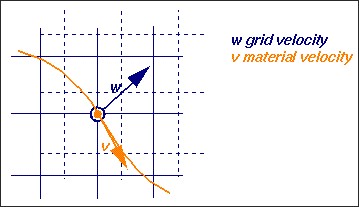
Рисунок 397: Произвольные скорости и смещения сетки

На практике встроенные алгоритмы определяют плавную деформацию сетки в соответствии со смещениями границ домена ALE. Доступно несколько алгоритмов (DONEA, SPRINGS, DISP и ZERO).

Стоит отметить, что формулировка ALE может быть вырождена в Лагранжевом (w=u: скорость сетки равна скорости материала) или в Эйлеровом (w=0: скорость сетки установлена ​​равной нулю).

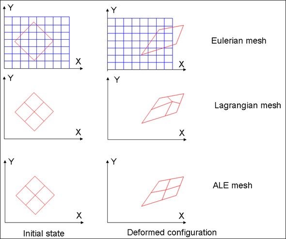
Рисунок 398: Сетки Эйлера, Лагранжа и ALE

Граничные узлы между материалами ALE и Лагранжа должны быть установлены на Лагранжевы: скорости сетки и материала равны. Граничные узлы между материалами ALE и Эйлера должны иметь скорость сетки, равную нулю.

Оба условия задаются с помощью параметра /ALE/BCS: можно указать расширенные граничные условия для узлов ALE (компоненты скорости сетки могут быть установлены на 0 или на скорость материала). Скорости сетки могут быть наложены с помощью связей ALE на любые узлы аналогично классическим кинематическим условиям (параметр /VEL/ALE в Engine).

Примечание: Когда твердый элемент соединен с элементом оболочки, соединенные узлы автоматически устанавливаются как Лагранжевы.

Соединение жидкости/конструкции

По крайней мере один ряд элементов ALE следует использовать, когда жидкость контактирует с оболочками.

Рисунок 399: Пример сетки для взаимодействия жидкости и конструкции

Методология

Цель этого раздела — показать несколько шагов для генерации правильной модели PRADIOS ALE/CFD.

Очистка CAD

Обычно человек получает модель CAD, по которой должна быть построена модель. Первая задача — очистить эту CAD и выполнить упрощения:

• Добавьте поверхности для закрытия объемов, используемых автоматической тетраэдрической сеткой

• Добавьте поверхность для управления прогрессией сетки

• Заплатите поверхности для подготовки зон сетки

  ◦ Удалите детали, размер которых меньше, чем можно решить

  ◦ Удалите линейные ограничения на поверхностях, когда это возможно

Создание сетки

Только элементы гексаэдра (или элементы квадрата в 2D-анализе) совместимы с формулировками ALE или Эйлера. Для создания сетки обычная техника заключается в том, чтобы сначала связать внешние поверхности каждой рассматриваемой области с треугольниками, затем автоматически сгенерировать внутреннюю объемную сетку тетраэдра и, наконец, разбить тетра на четыре гексаэдра каждый (внимательно следите за количеством элементов). Размер сетки треугольника должен быть в 3,5 раза больше запланированного размера сетки для тетраэдра.

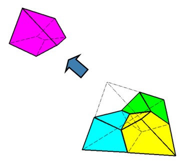
Рисунок 400: Тетраэдр, преобразованный в сетку гексаэдра

Эта функция переразметки находится в HyperWorks в разделе «split». Чтобы переразметить элемент тетраэдра в элемент гексаэдра, выберите split into hexas.

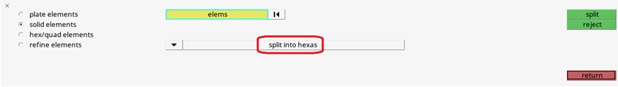
Рисунок 401:

Некоторые выдавливания добавляются при необходимости, например:

• Выход

• Вход

• Неотражающие границы (NRF)

• Трубы

Конечно, любая другая техника подходит для создания элементов гексаэдра.

Для граничных слоев размер элемента стены определяется, как описано в разделе Размер элемента стены. Сетка для граничного слоя обычно получается путем разбиения поверхности стены на треугольники. Затем, путем выдавливания сетки поверхности, создается сплошная сетка пентаэдра. Элементы пентаэдра можно впоследствии легко разделить на гексаэдры, как показано на рисунке 402.

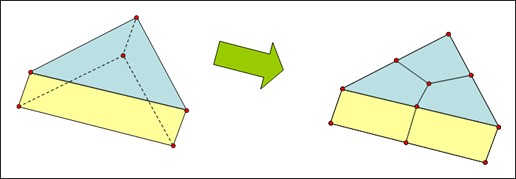
Рисунок 402: Разделение элемента пентаэдра на три гексаэдра

Определение характеристик сетки

При рассмотрении размера сетки учитываются два аспекта:

• Градиенты скорости и давления: вблизи турбулентных стенок размер сетки регулируется значением y+, которое может варьироваться от 100 до 1000 или даже выше (в трубах значения y+ до 8000 обеспечивают точные результаты). Оттуда геометрическая прогрессия обычно используется в направлении более грубых областей.

• Акустическая точность: максимальный размер может быть получен из минимальной длины волны, представляющей интерес. Обычно приемлемо использование 12 элементов на длину волны.

Очевидно, что первое условие будет управлять областью, близкой к препятствию или стене, а второе будет ограничивать максимальный размер во всей вычислительной области.

Для построения сетки обычно требуется некоторый компромисс. Общее время, Ttot, для моделирования можно оценить как:

\(Ttot ~20\cdot L/c\)

Где,

L

Самый большой размер модели

Общий необходимый ЦП, который является основным критерием для установления компромисса между осуществимостью и точностью, можно оценить как:

CPU = Ttot/dtc * Number of element * cpu/el/cycle

Генерация сетки для выполнения желаемого моделирования должна быть тщательно определена в соответствии с двумя критериями и компромиссом между осуществимостью (доступное время ЦП) и точностью.

Критерий 1: Адвекция

• 10 Минимальное количество элементов на вихрь для решения

• Локальное число Струхаля не более 1/6 для диапазона частот «интереса» в областях акустических источников:

  Str = f h/v < 1/6

  Например: fmax =600 Гц, v=30м/с ≥ h ~ 8 мм

Критерий 2: Акустическое распространение

• Критический в области, удаленной от акустических источников

• Шесть элементов на длину волны вдоль направления распространения

Например: fmax = 600 Гц, c=300 м/с ≥ h ~ 8 см

Компромисс

Между доступным общим временем ЦП для моделирования и критическим шагом времени; шаг времени будет автоматически установлен для удовлетворения условия Куранта:

dt = Min (h) / c

Общее время должно быть кратно наименьшей частоте, присутствующей в модели. Общее время ЦП пропорционально количеству циклов (конечное время, деленное на временной шаг), количеству элементов и стоимости каждого элемента (зависит от компьютера):

T = Ncycle * Nelem * Cost / cycle / elem

На практике рекомендуется выполнить хронометраж на паре циклов (не забудьте вычесть время инициализации), чтобы узнать стоимость цикла моделирования перед запуском большого моделирования.

Рассмотрим случай прохождения воздушного потока через препятствие (рисунок ниже), где целью моделирования является измерение шума, создаваемого этим потоком в любом месте сетки. Сетка должна иметь как минимум четыре различных области (см. Генерация сетки):

• Грубая сетка (вся вычислительная область, за исключением непосредственного окружения препятствия)

• Мелкая сетка (вблизи препятствия)

• Входной элемент (один ряд элементов)

• Выходные элементы (один ряд элементов)

При l — характерном размере препятствия в потоке, обычно есть три различные зоны сетки:

Зона	**Типичный размер элементов**	Примечание
очень хорошо	a	Выбранное таким образом препятствие дискретизируется минимум на 20 ячеек в каждом направлении.
хорошо	2a to 3a
course	4a to 6a	Убедитесь, что ячейки курса подходят для конвекции самых высоких частот интереса.

Если наибольшая частота, представляющая интерес в задаче, равна f, то ни одна ячейка в сетке не должна быть больше, чем:

Размер элемента < C / 10.f

Где,

C

Sскорость звука в жидкости

Толщина входного и выходного элемента должна составлять 1/10 соседних элементов расчетной области.

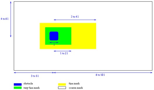
Рисунок 403: Количество элементов для типичной сетки для задач CAA (может различаться для конкретных приложений)

Для задач с низкими числами Маха (ниже 0,2) удовлетворительные результаты могут быть получены при предположении квазисжимаемости. Это сэкономит время на вычислениях. Сжимаемость подразумевает, что уравнения Навье-Стокса включают волновое уравнение. Тогда акустику и поток жидкости можно рассматривать одновременно, обеспечивая высокую численную точность. Квазисжимаемость означает, что транспортные члены, за исключением уравнения импульса, пренебрегаются. Поэтому, уменьшая C₁ в гидродинамических законах материалов, скорость звука уменьшается, а шаг по времени увеличивается (например, путем деления значения C₁ на 10, шаг по времени можно умножить на 3).

Интеграция по времени

Явная интеграция по времени на основе метода Ньюмарка является условно устойчивой. Условие Куранта также учитывает поток материала через элементы, что дает условие устойчивости:

\[\Delta t\leq S_{f}\ast\frac{\Delta t}{c+v-w}\tag{290}\]

\[v-w=\sqrt{\frac{1}{N}\sum_{i=1}^{3}\sum_{l=1}^{N}\left(v_{i}^{l} -w_{i}^{l}\right)^{2}}\tag{291}\]

Где,

N Количество узлов для рассматриваемых элементов

Масштабный коэффициент следует уменьшить до 0,7 и 0,5 для мультифизических законов.

Интеграция пространства

В целом, уравнение движения для поступательных скоростей с противопесочными часами и контактными силами записывается как:

\[M\frac{\partial v}{\partial t}=F_{ext}-F_{int}+F_{bod}+F_{hgr}+F_{cont}+F_{trm}\tag{292}\]

Где,

\(F_{trm}\) Вектор транспортного импульса задан как

\[F_{trm}=\sum_{element} f^{trm}\tag{293}\]

\[f_{il}^{trm}=(1+\eta_{I})\cdot\int_{v}\rho\cdot\Phi_{1}(w_{J}-v_{J})\cdot\frac{\partial v_{i}}{\partial x_{J}}dV\]

Все матрицы и векторы, определенные в приведенном выше уравнении, интегрированы по пространственной области. Массовая матрица не является постоянной во времени, поскольку плотность и область изменяются со временем. Показано, что решение уравнения является колебательным в пространстве, когда параметр сетки, известный как число Пекле, превышает критическое значение. Эту пространственную устойчивость можно избежать, добавив численную диффузию к схеме, которая в противном случае обычно является недодиффузионной и, таким образом, нестабильной. Коэффициент импульса восходящего потока определяется во входных данных материала. Полный случай восходящего потока (coef=1) является значением по умолчанию в PRADIOS и обычно используется.

В PRADIOS доступен один метод восходящего потока:

• Streamline Upwinding методом Петрова-Галеркина (SUPG):

SUPG заключается в изменении функций формы для учета терминов конвекции. Начиная с версии 2018 года, SUPG активирован по умолчанию. SUPG можно отключить с помощью параметра Engine file:

/UPWM/SUPG

Расчет сетки ALE

В формулировке ALE свобода перемещения сетки очень привлекательна, поскольку она помогает объединить соответствующие преимущества формул Лагранжа и Эйлера. Однако нелегко указать скорость сетки, хорошо подходящую для конкретной рассматриваемой задачи. Как следствие, практическая реализация описания ALE требует предоставления автоматического алгоритма предписания смещения сетки.

В PRADIOS существуют следующие автоматические расчеты сетки.

/ALE/GRID/DONEA

Это стандартный метод, применимый к большинству задач. Он основан на комбинации скоростей материала и сетки соседних узлов:

\[W_{J}(t+\Delta t/2)=\frac{1}{N}\sum_{J}W_{J}(t-\Delta t/2)+\frac{1}{N^{2}}\frac{\alpha}{\Delta t}\sum_{J}L_{IJ}(t)\sum_{J}\frac{u_{J}(t)-u_{J}(t)}{L_{IJ}(t)}\tag{295}\]

Где,

\[1-\gamma\leq\frac{W}{\nu}\leq 1+\gamma \tag{296}\]

N Количество узлов, подключенных к узлу

\(L_{IJ}\) Расстояние между узлом I и узлом J

a и\(\gamma\) Неразмерные факторы, заданные во входных данных

Следовательно, смещение сетки задается как:

\[u(t+\Delta t)=u(t)+w\left(\frac{t+\Delta t}{2}\right)\Delta t\tag{297}\]

/ALE/GRID/DISP

Формула среднего смещения вычисляет среднюю скорость для определения среднего смещения.

\[w(t+\Delta t)=\frac{1}{N}\sum_{J}W_{J}(t)\tag{298}\]

/ALE/GRID/SPRING

Каждый узел сетки соединен с соседними узлами сетки через нелинейную вязкую пружину, похожую на ту, что показана на рисунке 404.

Жесткость каждой пружины задается как \(M\Delta t_{02}\) (где, M — масса узла, а \(\Delta t_{02}\) — это типичный шаг времени, вводимый пользователем), можно определить вязкость и соотношение между жесткостью пружины на сдвиг и жесткостью пружин на растяжение-сжатие.

Следует отметить, что эти пружины влияют только на скорость узла сетки; они не влияют на скорость материала.

Этот метод очень точный и надежный, но очень дорогой с точки зрения процессорного времени.

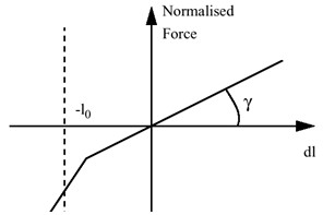
Рисунок 404: График силы пружины

/ALE/GRID/ZERO

Автоматический расчет сетки не выполняется. Скорость сетки либо постоянна (0, если начальная скорость сетки не указана, формуляция, следовательно, эйлерова), либо налагается свойством TYPE15 для деталей с движением жесткого тела.

Материалы ALE/CFD

Следующие законы материалов обычно используются для моделирования ALE/CFD с PRADIOS:

• Ньютоновская или турбулентная вязкая жидкость с моделью \(k-\varepsilon\) (активируйте LAW6 с помощью /MAT/K-EPS)

• Вязкая жидкость для вычислительной области моделирования больших вихрей (LES) (активируйте LAW46 с помощью /MAT/LAW46 (LES_FLUID))

• Элементарные граничные условия (активируйте LAW11 с помощью /MAT/LAW11 (BOUND))

• Элементарные граничные условия для турбулентного потока (активируйте LAW11 с помощью /MAT/B-K-EPS)

• Чисто термические материалы (активируйте LAW18 с помощью /MAT/LAW18 (THERM))

• Биматериал (активируйте LAW20 с помощью /MAT/LAW20 (BIMAT))

• Гидродинамическая биматериальная жидкость-газ (активируйте LAW37 с помощью /MAT/LAW37 (BIPHAS))

• Многоматериальное твердое тело, жидкость и газ (активируйте LAW51 с /MAT/LAW51 (MULTIMAT))

• Многожидкостный твердый, жидкий и газообразный (LAW151 активирован с /MAT/LAW151 (MULTIFLUID))

Многие параметры уже определены по умолчанию и обеспечивают точные результаты. Вам не нужно переопределять эти параметры, но вы можете настроить физические свойства, соответствующие материалу и единицам, которые вы используете.

Турбулентность с \(k-\varepsilon\) Модель

Основная идея турбулентности (уравнения Рейнольдса) состоит в том, чтобы разделить фактическую скорость жидкости на ее среднюю составляющую и ее флуктуации; флуктуации скорости предполагаются малыми по отношению к средней скорости. Тогда изотропная теория турбулентности демонстрирует эквивалентность этих предположений и введение дополнительного вязкого члена в турбулентную вязкость (приближение Буссинеска).

Материал L.E.S.

Модели турбулентности, основанные на уравнениях Рейнольдса, разделяют средние величины от флуктуаций и по замыслу вынуждают к решению устойчивого состояния.

Всякий раз, когда поток содержит крупные структуры, флуктуации нельзя пренебречь по сравнению со средними величинами. Тогда уравнения Рейнольдса не могут точно обрабатывать такие ситуации.

Моделирование больших вихрей (LES) отличается. Не выполняется поиск стационарного состояния или среднего потока. Предполагается, что сетка сетки частично разрешает турбулентность. По крайней мере, макроструктуры, тогда как меньшие масштабы заменяются вязким членом (масштаб подсетки), который, как предполагается, моделирует в основном диссипативные эффекты микротурбулентности.

Материал LAW46 предназначен для моделирования больших вихрей. PRADIOS можно использовать с моделью масштаба подсетки Смагоринского: (\(I_{sgs}\) =1 или 2) или без: (\(I_{sgs}\) =0) (подход MILES). Уравнение состояния линейно сжимаемо (постоянная сжимаемость), хорошо подходит для дозвуковых случаев. Все элементы, подключенные к узлу, как фиксированные, так и лагранжевые, будут автоматически рассматриваться как элементы стенки, а их вязкость будет задана в соответствии с логарифмическим профилем скорости.

Необходимо указать плотность, скорость звука, молекулярную кинематическую вязкость, тип модели масштаба подсетки (рекомендуется TYPE2) и константу масштаба подсетки (по умолчанию 0,1).

В таблице ниже приведены различные материалы, доступные для различного использования.

√ : да; пусто: нет

См. также

Материалы/Отказ (FAQ)

Квазисжимаемый вариант

Для квазисжимаемой опции предполагается, что плотность и энергия постоянны.

Конвекция-диффузия не вычисляется:

\[\frac{\partial\rho}{\partial t}=-\rho\nabla\mathbf{u}\tag{299}\]

Поэтому производительность повышается и требуется меньше времени для вычислений.

Квазисжимаемая опция может быть активирована в файле PRADIOS Engine с помощью /INCMP.

Используя эту опцию, акустические волны распространяются так же точно, как и в сжимаемом случае. Однако ее нельзя объединить с \(k-\varepsilon\) моделью турбулентности.

Турбулентная стенка

Элементы турбулентной стенки определяют замыкание системы с \(k-\varepsilon\) моделью диффузионных уравнений.

Условия турбулентной стенки задаются автоматически в элементах, имеющих по крайней мере один узел с фиксированными граничными условиями (111 … … …) или с условиями Лагранжа (… … … 111).

Условия Лагранжа должны быть явно объявлены во входных данных PRADIOS для свободных узлов, соединенных с оболочками; хотя эти узлы, очевидно, являются Лагранжевыми.

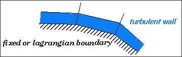
Рисунок 405:

Незадание узловых граничных условий на границах стенок системы может привести к неопределенности и расхождению. Использование модели \(k-\varepsilon\) подразумевает, что в вашей задаче должна быть хотя бы одна турбулентная стенка.

Размер элемента стенки

Обычно значение \(\gamma_{2}^{+}\) считается критическим, и для трубок вы получаете хорошие результаты для значений \(\gamma_{2}^{+}\) вплоть до 3000. Разумные значения находятся между 100 и 1000. Где,

\[y_{2}^{+} = \left(u^{*}y_{2}\right)/v\tag{300}\]

Ult,

\(u^{*}\) Скорость трения

\(\gamma_{2}\) Размер элемента, перпендикулярного стенке

v Ламинарная кинематическая скорость

В PRADIOS \(\gamma_{2}^{+}\) также равна:

\[y_{2}^{+} = 4.77\left(\frac{v_{t}}{v}\right)\tag{301}\]

Где \(v_{t}\) — турбулентная кинематическая вязкость.

Как правило, сетки строятся с учетом доступности с некоторым компромиссом по значению \(\gamma_{2}^{+}\). Если это значение слишком велико, это означает, что пограничный слой будет плохо интегрирован. Для открытых случаев, когда пограничный слой часто отрывается, размер сетки в следе за телом в основном определяется размером вихрей. В этом случае можно думать, что точность определяется не размером элемента стенки, а качеством алгоритма.

Узловые граничные условия

По умолчанию кинематические ограничения действуют на скорости и ускорения материалов. В PRADIOS вы можете определить широкий спектр таких ограничений. Для мультифизических и жидкостных приложений возможны следующие варианты:

• Фиксированные и полные граничные условия скольжения

• Наложенные скорости (наложенный поток на входе)

• Жесткие связи (временные добавления при перезапусках)

• Жесткие тела для моделирования жестких конструкций и соединений, а также для расчета сил сопротивления и подъема (импульс жидкости на твердом теле хранится в базе данных истории времени)

Ограничения сетки действуют только на скорости сетки. Укажите:

• Фиксированные и полные условия сетки скольжения

• Лагранжевы условия (скорость сетки и материала задаются одинаково)

• Связи ALE для поддержания регулярного распределения узлов

• Наложенные скорости сетки (движущиеся вход и выход)

Если фиксированный узел с /BCS, то это означает, что сетка и материал фиксированы. Если используется /ALE/BCS, то это другое. Первые 3 кода определяют сетку DOF, вторые 3 кода определяют, если узел действует как Лагранжев в соответствующем направлении.

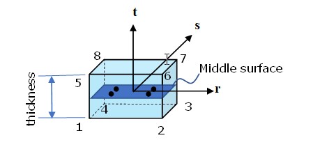
Рисунок 406:

Пример:

Если установлено Grilag=010 000, это означает, что просто фиксируется сетка в направлении Y, материал может перемещаться в направлении Y.

Если установлено Grilag=000 010, это означает, что узлы подобны лагранжевым в направлении Y, сетка и материал привязаны к этим узлам в направлении Y.

Если установлено Grilag=010 010, это означает, что сетка и материал привязаны к этим узлам в направлении Y и зафиксированы в направлении Y. Это похоже на trarot=010 000 в /BCS. .. image:: vertopal_7197fe79ded4471fa6ba70c4c62a5530/media/image164.jpg

width

7.33397in

height

2.26686in

Рисунок 407:

Элементарные граничные условия

Граничные элементы позволяют задавать значения элементов на границах домена. Их можно задать двумя способами:

Один с граничными элементами (квадраты в 2D-анализе и твердые тела в 3D-анализе) с материалом:

• /MAT/LAW11

• /MAT/LAW51

• /MAT/LAW18 (в случаях чисто термического материала)

Другой способ — назначение /EBCS на поверхности граничных элементов.

Для каждой переменной P, rho, T, k, epsilon, внутренней энергии можно задать следующее:

• наложенные изменяющиеся условия в соответствии с пользовательской функцией

• непрерывность

• плавно изменяющаяся предопределенная функция

С PRADIOS ALE/CFD можно указать любую комбинацию из указанных выше опций; с другой стороны, замыкание различных уравнений конвекции и диффузии должно быть тщательно проверено вами.

Обычно используются следующие типы элементарных граничных условий:

• Вход:

Поток накладывается с использованием наложенных скоростей /IMPVEL; плотность, энергия, турбулентная энергия (то есть: k) накладываются как константы. Непрерывность накладывается на давление (только для отображения) и для эпсилон. Турбулентная энергия, rho k устанавливается на ноль для внешних потоков и на 1,5*rho*(0,06 V_in)² для внутренних потоков.

• Выход:

Непрерывность для всех переменных, кроме давления, которое накладывается. При использовании опции Неотражающие границы (NRF) вы указываете значение для скорости звука и типичной длины релаксации, которая должна быть больше, чем наибольшая длина волны, представляющая интерес.

• Стороны:

Непрерывность для всех переменных с опцией Non-reflective frontiers (NRF) или условиями скольжения без граничных элементов. Это обеспечивает свободное сопротивление поля полям давления и скорости.

Если элемент не существует на границе, предполагается непрерывность; но необходимы кинематические условия, чтобы запретить потоки; в противном случае уравнение конвекции не замкнуто, и программа может расходиться.

Указать элементарные переменные на границе вычислительной области. - В Material LAW11 ниже используются следующие параметры:

◦ Ityp = 0 определяет условия стагнации для идеального газа (вход Бернулли).

◦ Ityp = 1 определяет условия стагнации для линейного сжимаемого материала (вход Бернулли).

◦ Ityp = 2 устанавливает значения (вход/выход).

◦ Ityp = 3 для неотражающих границ (выход).

• В материале LAW51 использованы следующие варианты:

◦ Iform= 2 позволяет накладывать субматериальные состояния (плотность, энергия и объемная доля), которые также используются для вычисления глобального материального состояния. (вход).

◦ Iform= 4 условия входа газа для многоматериальных законов ALE (стагнация входа газа).

◦ Iform= 5 условия входа жидкости для многоматериальных законов ALE (стагнация входа жидкости).

◦ Iform= 6 Этот граничный материал позволяет моделировать неотражающую границу выхода для многоматериального закона /MAT/LAW51 (выход NRF).

Например, во входной колоде плотность и энергия накладываются постоянными на входе. Неотражающие границы накладываются на выходе. Затем поток вводится на входе через наложенные скорости в узловых точках.

Неотражающие границы (NRF)

Ityp=3 в LAW11 и Iform=6 в LAW51 используются для предотвращения отражений исходящих волн на границах области.

Две возможности:

• Среднее давление накладывается через функцию. Добавляется релаксационный член, чтобы среднее давление сходилось к наложенному значению. Это хорошо подходит для выходов.

• Среднее давление рассчитывается из давления соседнего элемента, и давление сходится к этому постоянно меняющемуся значению.

Сопротивление границы в точности равно волновому сопротивлению монополя, излучающего на расстоянии \(2l_{c}\) от границы, где \(l_{c}\) указано во входных данных для этого закона.

Эти неотражающие границы (NRF) неэффективны, когда скорости наложены или когда узлы фиксированы.

Искусственное демпфирование для ударных волн

Квадратичная объемная вязкость \(\mathrm{q_{a}}\) и линейная объемная вязкость \(\mathrm{q_{b}}\) по умолчанию установлены на значения, релевантные для гидродинамики и задач высокоскоростного удара, включающих ударные волны.

Для динамики жидкости и акустики эти коэффициенты не требуются, и обычно устанавливаются на очень малые значения, чтобы переопределить значения по умолчанию.

Кинематические ограничения

Доступны два вида кинематических условий: - Условия, применяемые к материальным скоростям

• Условия по скорости сетки (ALE)

По умолчанию все кинематические условия применяются к материалу, а не к сетке. Для приложений ALE интерес представляют следующие опции:

• Фиксированные и полные граничные условия скольжения

• Наложенные скорости (например: наложенный поток на входе)

• Жесткие связи (временные добавления при перезапусках)

• Жесткие тела для моделирования жестких конструкций и соединений, а также для вычисления сил сопротивления и подъема (то есть импульс жидкости на твердом теле сохраняется в базе данных истории времени).

Граничные условия

Граничные условия ALE активируются с помощью ключевого слова /ALE/BCS в входной колоде. Ограничения сетки действуют только на скорости сетки. Если граничное условие не указано для скорости сетки, узлы могут перемещаться любым произвольным образом (ALE).

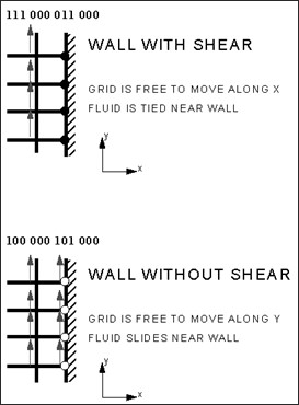
Рисунок 408: Приложения граничных условий ALE

Жесткое тело (/RBODY)

Жесткое тело определяется основным узлом M и набором вторичных узлов. Жесткие тела используются в приложении CFD для вычисления реактивных сил на конструкциях.

Связи ALE (VEL/ALE)

Связь ALE представляет собой набор из n узлов со скоростью сетки, контролируемой двумя основными узлами M1 и M2. Входные данные вводятся при каждом перезапуске (временное добавление). Доступны три варианта:

• Скорость линейно интерполируется относительно порядка ввода

• Скорость устанавливается на максимальную абсолютную скорость основных узлов

• Скорость устанавливается на минимальную абсолютную скорость основных узлов

Интерфейсы

Доступные алгоритмы контакта в PRADIOS представлены в Таблице 24.

Таблица 24: Интерфейсы PRADIOS Face-to-Face

Nbg	Описание	Приложение	Контакт Уход
1 & 9	ALE / LAG с раздвижным	Жидкость- взаимодействие структура	Основное- Вторичное
2	Связанный интерфейс	Изменение сетки плотности (сплошная)	Основное- Вторичное или LM
3 & 5	Контактное воздействие между 2-мя част.	Use of type 7 is recommended	штраф
6	Контактное воздействие между 2-мя твердые тела	Пользовательские контакты	штраф
7	Общее назначение контактное воздействие между 2-мя частями	Твердый контакт воздействие на все скорости	штраф или LM
8	Вытяжка контакта	Штамповка приложения	штраф
10	Похоже на: тип 7, но привязанный контакт	Специальное назначение интерфейса	штраф
11	Влияние между 2-х линий	Для балок, стержни или пружины	штраф
12	Жидкость / жидкость контакт	Жидкость в Жидкость контакт	штраф
16 & 17	контакт между узлами квадратичной формы и твердые оболочки или между квадратными формами	Сетки с 8 или 16 узлами толстостенный или 20 блочный	LM
18	CEL Lagrange / Euler interface	Взаимодействие жидкости и структуры	штраф
22	Lagrange поверхность и Жидкостная область	Взаимодействие жидкости и структуры	штраф

Конкретные интерфейсы для приложений PRADIOS ALE/CFD:

• TYPE1: для связи части ALE с частью Лагранжа

• TYPE12: для блоков ALE/Эйлера для связи с подвижными или фиксированными сетками

• TYPE18 и TYPE22: для обработки взаимодействий жидкость-конструкция

Интерфейс жидкость/жидкость

Интерфейс TYPE12 предназначен для соединения двух несоответствующих сеток. Его использование ограничено основным/вторичным подходом, то есть не более одного основного узла подключено к вторичному сегменту.

Примечание: Основной/вторичный алгоритм поиска может не сработать там, где есть острые углы. В этом случае необходимо разделить интерфейс на несколько интерфейсов.

Вы также можете обнаружить ошибку, когда ближайший основной узел данного вторичного узла не принадлежит сегменту перед вторичным узлом. В этом случае настройте сетку локально, чтобы избежать неоднозначных ситуаций.

Интерфейс доступен для параметров квазисжимаемости и сжимаемости.

Выберите главную и вторичную стороны в интерфейсе Fluid/Fluid (тип 12)

Правило 1:

Каждому вторичному узлу нужен основной сегмент.

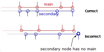
Рисунок 409:

Это должно оставаться верным при перемещении интерфейса.

Если узел не имеет проекции на основную поверхность, алгоритм выдает предупреждение, но все равно работает, поскольку вторичный узел остается связанным с ближайшим основным сегментом.

Правило 2:

Каждый основной узел должен получать вклад как минимум от вторичного узла.

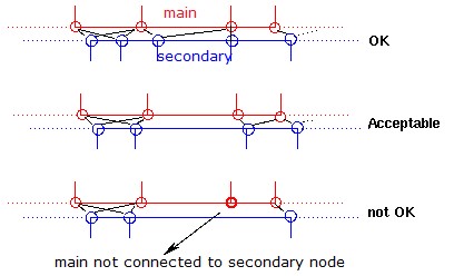
Рисунок 410:

Если у основного сегмента нет вторичного, но у его соседей есть, алгоритм все равно работает, поскольку приведенное выше правило выполняется. В принципе, тем не менее, рекомендуется, чтобы основные сегменты имели по крайней мере один вторичный узел.

Можно сказать, что вторичная сетка должна быть тоньше или равна основной.

Правило 3:

При сжимаемости любой сегмент (основной или вторичный) должен быть поверхностью одного и только одного элемента ALE-кирпича.

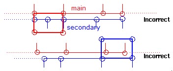
Рисунок 411:

Правило 4:

Кинематические условия на вторичной стороне допускаются только если соответствуют идентичным условиям на главной стороне.

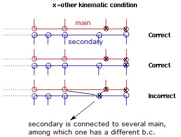
Рисунок 412:

Это должно оставаться верным, когда интерфейс скользит.

Взаимодействие жидкости/конструкции (интерфейс ALE/Лагранжа)

Доступны три вида интерфейсов.

Интерфейс TYPE1

Интерфейс TYPE1 используется для определения границ между доменами ALE и Лагранжа. Условия полного скольжения применяются на границе между двумя доменами, как полная скользящая стенка. Нормальные скорости материала узлов Лагранжа и ALE устанавливаются одинаково.

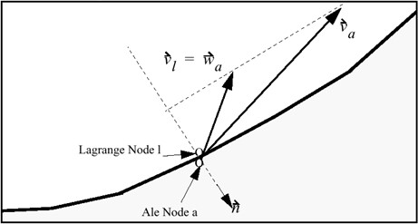
Рисунок 413: Взаимодействие жидкости и конструкции с интерфейсом TYPE 1

Интерфейс TYPE9

Это интерфейс ALE/Лагранжа с пустотным отверстием и свободной поверхностью (то есть, если основная и вторичная стороны не соприкасаются, то взаимодействия между ними нет). Часть ALE определяется как вторичная, а часть Лагранжа определяется как основная. Скорость сетки равна скорости материала в нормальном направлении.

Интерфейс TYPE18 (CEL)

Интерфейс TYPE18 создает контакт между узлами Эйлера/ALE и основной поверхностью Лагранжа. Метод вязкоупругого штрафа используется для наложения относительной скорости материала (жидкости), касательной к основной поверхности. Скорость сетки не изменяется этим интерфейсом. Интерфейс позволяет моделировать проникновение лагранжевой части (структуры) в сетку Эйлера/ALE, например, в случае столкновения кораблей.

Качество результатов моделирования с использованием этого интерфейса сильно зависит от параметров интерфейса и, в особенности, от его жесткости.

Рекомендуемый коэффициент жесткости интерфейса для задач взаимодействия жидкости и конструкции можно получить следующим образом:

\[\mathit{Stfac}=\frac{\rho\cdot v^{2}\cdot S_{el}}{Gap}\tag{302}\]

Где,

\(\rho\) (Наивысшая) плотность жидкости

v Скорость явления (скорость звука или выше для сверхзвукового явления)

\(S_{el}\) Поверхность элементов Лагранжа

Для аэродинамических задач рекомендации следующие:

• \(Gap=1.5L_{c}\) with \(L_{c}\) being the length of fluid element

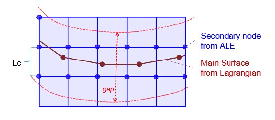
Рисунок 414:

• Постоянная жесткость с \(K=g\cdot P\cdot L_{c}\)

• Вязкость, связанная с жесткостью интерфейса:

\[v_{s}=2a\cdot Gap^{2}\cdot\sqrt{yP\rho}\tag{303}\]

С \(\alpha=0.5\) или \(\alpha=\gamma\)

P и \(\rho\) являются характеристиками воздуха

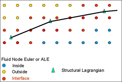
Рисунок 415: Взаимодействие жидкости и конструкции с интерфейсом ТИПА 18

Рекомендуемое значение зазора равно 1,5 по размеру элемента.

Примечание: Интерфейсу нужна достаточно мелкая сетка, чтобы обеспечить соответствующие результаты.

Единицы измерения

PRADIOS имеет встроенную систему единиц измерения, чтобы вы могли предоставлять данные в любой согласованной системе.

Для проверки согласованности проверьте, что давление = плотность x длина²/ время²

Самые популярные единицы измерения (с примерами из стали):

Длина	Time	Стресс	Mass	Force	Энергия	Плот- ность	модуль Янг	Гра- вита- ция	Предел теку- чести
m	s	Pa	kg	N	J	7.8 e+03	2.1 e+11	9 .81e +00	2.06 e+05
mm	ms	MPa	g	N	mJ	7.8 e-03	2.1 e+05	9.81 e-03	2.06 e+02
mm	ms	GPa	kg	KN	J	7.8 e-06	2.1 e+02	9.81 e-03	2.06 e-01
mm	s	MPa	Mg (ton)	N	mJ	7.8 e-09	2.1 e+05	9 .81e +03	2.06 e+02
cm	micros	Mbar	g	\(1 0^{7}\) N	\(1 0^{5}\) J	7.8 e+00	2.1 e+00	9.81 e-10	2.06 e-06

См. также

/UNIT (Стартер)

Вход двигателя

В качестве примера, следующие параметры панели двигателя могут использоваться в PRADIOS CFD.

Определение дополнительных команд для управления шагом времени

/DT/BRICK/STOP
1. 1.E-6
/DT/SHELL/CST
0.9 1.E-5

Определите команды для определения ваших вариантов вывода Файл истории времени

/TFILE                  Интервал вывода
1.e-4

Файл вывода двигателя

/PRINT/100              Интервал цикла для вывода

Анимация

/ANIM/DT                     настройки времени
0.09 0.000833                время для первого файла анимации, интервал

Выбор элементарных переменных

/ANIM/ELEM/K            Турбулентная энергия
/ANIM/ELEM/TVIS         Турбулентная вязкость
/ANIM/ELEM/P            Давление

Выбор узлового вектора

/ANIM/VECT/VEL  скорость
/ANIM/VECT/DISP смещение

Отфильтрованный выборочный вывод

/@TFILE
0. 1.E-4 Время начала, интервальные узлы
2009 2010 2011 2012 2017 2018 2023 2024 2029 2030
2035 2036 2041 2042 2047 2048 2053 2054 2059 2060
2065 2066 2071 2072 2077 2078 2153 2154 2157 2158
2161 2162 2165 2166 2169 2170 2173 2174 2177 2178
.....#

Устранение неполадок

Программа обычно дает сбой, когда:

• Останавливается с плавающей ошибкой исключения

• Временной шаг быстро уменьшается

В большинстве случаев сбой программы вызван:

• Расхождение

• Возбуждение песочных часов

• Несовместимое граничное условие

Рассматривая кривые временной истории, такие как кинетическая энергия, турбулентная энергия, вращательная энергия, энергия песочных часов, материальные переменные и т. д., попытайтесь определить время, когда может наблюдаться неожиданное поведение.

Если Starter не выдает четкое сообщение, откройте выходной файл и найдите слово "ERROR", которое определит более подробное объяснение проблемы. If Starter crashes, open the Starter output (Rootname_0000.out) file and go to the end. Review the data to see if it makes sense or not - most likely ‘not’. Then go backwards until you find data that does makes sense. Go to your input deck and inspect the area close to the switch between what makes sense and what does not make sense. There might be too many or not enough cards there.

Примечание: Любое изменение в колоде входных данных должно бытьотражено в контрольных картах, если это необходимо.

Если двигатель останавливается из-за отрицательной плотности или проблемы с временным шагом или происходит сбой:

• Повторно выполните перезапуск между вашим последним файлом перезапуска и «прямо перед расхождением»

• Выполните новый перезапуск до расхождения со следующими параметрами в файле Engine:

/PRINT/-1 /ANIM/DT Ti 1.E-30 (где Ti — начальное время этого запуска + эпсилон) /TFILE/ 1.E-30

Затем у вас будет распечатка в листинге, файл анимации и образец истории времени для каждого цикла. Используйте их для исследования вашей проблемы. Очень часто, глядя на поле скорости в анимации, выявляется некоторая нерегулярность; которую можно легко связать с дырой в граничных условиях.

Расхождение

Дивергенция означает, что какая-то переменная становится слишком большой. Это может произойти, если ваша проблема плохо определена (математически) или если временной шаг больше, чем теоретический критический временной шаг (численный).

Попробуйте локализовать проблему во времени и пространстве, запустив программы истории времени и анимации. Ищите аномальные скорости, турбулентную энергию и вязкость.

Проверьте свои границы:

• Кинематические ограничения

• Элементарные границы (материал TYPE11)

Проверьте классические предположения механики жидкости.

Поищите утечки в вашей сетке (несовпадающие узлы, неплоскостные симметрии, пропущенные граничные условия). Если используется модель турбулентности, проверьте, есть ли у вас хотя бы одна турбулентная стенка.

Поищите модели скорости в виде песочных часов. Это может произойти, если у вас концентрированные потоки, элементы с плохими пропорциями или если коэффициент песочных часов установлен на очень малое значение (см. параметры материала).

Проверьте, чтобы убедиться, что у вас нет оболочки толще, чем размер элемента: изгибная устойчивость является приоритетом, предполагаемым в коде (не рассчитываемым), и это предположение является консервативным только до тех пор, пока толщина не превышает длину оболочки.

Гидродинамика гладких частиц (SPH)

Формулировка метода гидродинамики гладких частиц используется для решения уравнений механики, когда частицы свободны от сетки.

Он специально адаптирован для моделирования явлений с очень существенной деформацией, то есть диапазона приложений, где метод конечных элементов с формулировкой ALE и Лагранжа теряет свою эффективность и точность.

Метод SPH, встроенный в код PRADIOS, совместим с большинством функций. Например, можно заставить взаимодействовать два объекта, один из которых дискретизирован конечными элементами, а другой — частицами.

Формулировку SPH можно поместить в модель ALE, только если граница между SPH и ALE является лагранжевой. Формулировка SPH доступна только в 3D-анализе.

См. также

RD-E: 1300 Эксперимент с ударной трубой

RD-E: 2200 Затопление

RD-E: 4900 Удар птицы о лобовое стекло

RD-E: 5500 Инициализация вращения лопасти вентилятора и воздействие

Распределение ячеек SPH (Руководство по теории)

Распределение ячеек SPH

Частицы должны быть созданы в гексагональной компактной, гранецентрированной кубической или кубической сетчатой ​​упаковке.

Гексагональная компактная сетка и гранецентрированная кубическая упаковка рекомендуются для использования в PRADIOS и дают схожие результаты. Распределение кубических частиц по центру грани можно создать с помощью панели HyperMesh SPH. Макрос HyperMesh Tcl для создания гексагональной компактной сети доступен на веб-сайте Laduga Connect.

Гексагональная компактная сеть

Кубическая центрированная сетка граней реализует гексагональное компактное распределение, которое может быть полезно для построения сетки.

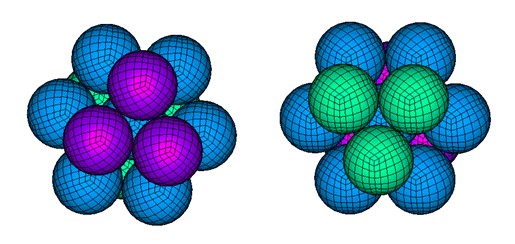
Рисунок 416: Локальные виды гексагональной компактной сети

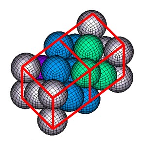
Рисунок 417: Перспективный вид кубической центрированной сетки граней

Распределение гексагональной компактной сетки можно создать в HyperMesh с помощью скрипта Tcl, доступного при поиске в Laduga Connect для скрипта Tcl Hexagonal Compact Net. При использовании этого скрипта шаг или расстояние между любой частицей и ее ближайшим соседом вводится как h₀.

Масса частицы m_*p* определяется в свойстве /PROP/SPH.

Масса частицы SPH связана с плотностью материала \(\rho\) и шагом h₀ гексагональной компактной сетки. Эта масса частицы может быть рассчитана как:

\[m_{p}\approx\frac{h_{0}^{3}}{\sqrt{2}}\rho \tag{304}\]

Поскольку пространство можно разбить на многогранники, окружающие каждую частицу сети, каждая из которых имеет объем:

\[V_{p}=\frac{h_{0}^{3}}{\sqrt{2}}\tag{305}\]

Из-за различий в дискретизации объема массу можно более точно представить как:

\[m_{P}=\frac{\rho V}{n}\tag{306}\]

Где,

V Общий объем, заполненный частицами.

n Общее количество частиц, распределенных в объеме.

Для гексагональной компактной сети рекомендуемая длина сглаживания h в /PROP/SPH — это шаг h₀, который является наименьшим расстоянием между частицами. Длина сглаживания, меньшая, чем эта, может использоваться только в том случае, когда нет физических проблем с растяжением материала. Если материал включает в себя поведение при растяжении, то длина сглаживания, большая, чем h₀, может использоваться для повышения устойчивости, но это приведет к увеличению вычислительных затрат.

В следующей таблице показано количество соседей при использовании различных длин сглаживания h в /PROP/SPH. Точность и вычислительные затраты моделирования улучшаются по мере увеличения длины сглаживания.

Таблица 25: Количество соседей в гексагональной компактной сети

Расстояние d	Номер частицы на расстоянии d	Номер частицы на расстоянии без d
\(h_{o}\)	12	12
\(\sqrt{2}h_{2}\)	6	18
\(\sqrt{3}h_{2}\)	24	42
\(2h_{o}\)	12	54
\(\sqrt{5}h_{2}\)	24	78

Гранецентрированный куб

Гранецентрированный куб располагает частицы в группах по 14, образуя углы и центр каждой грани куба.

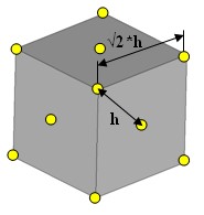
Рисунок 418:

Подобно гексагональной компактной сетке, каждая частица имеет 12 соседей, а масса частицы равна:

\[m_{P}=\frac{\rho V}{n}\tag{307}\]

Для гранецентрированной кубической сетки рекомендуемая длина сглаживания h в /PROP/SPH — это шаг, введенный при создании сетки sph в HyperMesh. Шаг h₀ — это наименьшее расстояние между частицами. Длина сглаживания, меньшая, чем h₀, может использоваться только тогда, когда нет физических проблем с растяжением материала. Если материал включает поведение растяжения, то длина сглаживания, большая, чем h₀, может использоваться для повышения устойчивости, но это приведет к увеличению вычислительных затрат.

Простая кубическая сетка

Let, c the side length of each elementary cube into the net.

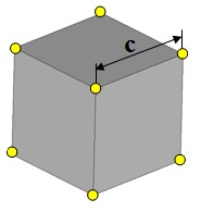
Рисунок 419:

Масса частиц \(m_{p}\) должна соотноситься с плотностью материала \(\rho\) и размером c сети, согласно следующему уравнению:

\[m_{P}=c^{3}\rho \tag{308}\]

Таблица 26: Количество соседей в кубической сети

Расстояние d	Номер частицы на расстоянии d	Номер частицы на расстоянии без d
c	6	6
\(\sqrt{2}c\)	12	18
\(\sqrt{3}c\)	8	26
2c	6	32
\(\sqrt{5}c\)	24	56
\(\sqrt{6}c\)	24	80
\(\sqrt{2}c\)	12	92
3c	6	98

Из опыта использования кубической сети, для решения проблемы неустойчивости натяжения требуется более высокая длина сглаживания по сравнению с гранецентрированной кубической или гексагональной компактной сетью. Эта более высокая длина сглаживания увеличивает вычислительные затраты, поскольку в расчет для каждой частицы необходимо включить больше соседних частиц.

Для кубической сети в /PROP/SPH рекомендуется длина сглаживания h между 1,25c и 1,5c.

Максимальное хранимое количество соседей

Когда в пределах безопасного расстояния обнаруживается более Nneigh соседей, программа сохраняет только Nneigh ближайших точек и уменьшает значение \(\alpha_{sort}\).

Если все истинные соседи, лежащие внутри сферы влияния всех частиц, все еще сохраняются, то результаты не меняются.

В другом случае сообщение типа "Предупреждение о вычислении SPH" отправляется в выходной файл PRADIOS. Обратите внимание, что в случае такого сообщения время вычисления увеличивается, поскольку становится необходимым сортировать ближайшие частицы на каждом цикле. Более того, такую ​​ситуацию необходимо тщательно анализировать, поскольку она часто приводит к очевидной (локальной) неустойчивости.

Условия симметрии SPH

Условия множественной симметрии SPH

Условие аксиальной симметрии можно смоделировать с помощью двух условий относительно двух плоскостей, пересекающихся по оси симметрии. Условие сферической симметрии можно смоделировать с помощью трех условий относительно трех плоскостей, пересекающихся по центру симметрии.

Тем не менее, эти виды симметрии обрабатываются по-разному.

Например, в случае условия аксиальной симметрии не все призрачные частицы строятся вокруг оси симметрии. Строятся единственные симметричные частицы реальных частиц относительно двух плоскостей симметрии.

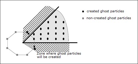
Рисунок 420: Неполные множественные симметрии

Следовательно, некоторые характеристики условий аксиальной симметрии (соответственно сферической симметрии) могут быть близки к оси симметрии (соответственно центру симметрии).

Узлы, близкие к оси симметрии (соответственно центру симметрии) и лежащие на плоскости симметрии (P), могут получить нормальную к (P) скорость, которая не равна нулю, поскольку их окрестность не симметрична относительно плоскости (P).

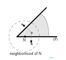
Рисунок 421: Окрестность частицы N не симметрична относительно плоскости (P), и нормальная скорость N к плоскости (P) может быть ненулевой

Кинематическое граничное условие

В отношении предыдущего обсуждения: добавление кинематического граничного условия явным способом позволяет обеспечить его соблюдение.

Кинематическое граничное условие будет добавлено к узлам, принадлежащим группе узлов, указанной в опции /SPHBCS, так что:

• Если тип “Slide”, скорость узла в направлении “Dir” устанавливается на ноль

• Если тип “Tied”, скорость узла во всех направлениях устанавливается на ноль

В случае нескольких кинематических граничных условий, примененных к одному и тому же узлу через различные условия симметрии SPH, кинематические граничные условия составляются автоматически, даже если кинематические граничные условия применяются в неортогональных направлениях.

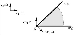
Рисунок 422: Комбинация кинематических граничных условий из различных условий симметрии SPH

Рисунок 422 показывает, что если два кинематических граничных условия применяются к N через два условия симметрии относительно плоскостей (P₁) и (P₂), два граничных условия изменяются так, что скорость в плоскости, нормальной к общей оси (P₁) и (P₂), останется нулевой. Обратите внимание, что если одно из двух условий симметрии является условием типа «Связано», скорость N во всех направлениях устанавливается равной нулю.

Он также позволяет применять к одному и тому же узлу кинематическое граничное условие через условие симметрии SPH (/SPHBCS) и стандартное граничное условие (/BCS) одновременно, пока стандартное граничное условие не задано в подвижной системе скоса, а в фиксированной системе скоса или глобальной системе скоса. Затем эти два условия составляются одинаковым образом.

Часть Масса

Вам следует знать, что когда частица лежит на плоскости симметрии в момент времени t=0, масса и начальный объем, рассматриваемые для частиц, соответственно:

\[m=\frac{m_{P}}{2},\quad V=\frac{m_{P}}{2\rho}\tag{309}\]

Где, \(m_{p}\) — это масса, указанная в наборе свойств.

Когда частица лежит на n плоскостях симметрии в момент времени t=0,

\[m=\frac{m_{P}}{n},\quad\quad V=\frac{m_{P}}{n_{\rho}}\tag{310}\]

Частицы-призраки, построенные из этой частицы, получат тот же начальный объем и массу.

Когда n>2, предыдущее уравнение может давать ошибку в массе и энергии выходе для части, к которой принадлежат частицы, относительно физической модели.

Уровень формулировки

Когда определена плоскость симметрии, и даже если кинематическое условие установлено для всех частиц, лежащих на плоскости симметрии, частицы, лежащие в нулевой момент времени внутри домена, теоретически могут пересекать плоскость симметрии.

Это характерно для SPH, для которого жесткость между частицами не возрастает до бесконечного значения, когда частицы коллапсируют. Поэтому это может произойти, когда частицы, лежащие на плоскости симметрии, позволяют частицам, которые находились внутри домена, проходить через плоскость симметрии.

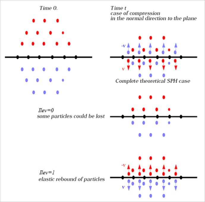
Рисунок 423: Уровень формулировки

Если Ilev=0, частицы, пересекающие плоскость симметрии, будут (постепенно) больше не учитываться в расчетах, как и их симметричные частицы, которые затем лежат внутри области.

Если Ilev=1, частицы, пересекшие плоскость симметрии, упруго отскакивают от плоскости симметрии: их скорость в направлении, нормальном к плоскости, устанавливается противоположной.

Примечание: Когда Ilev=1, настоятельно рекомендуется связать кинематическое условие со всеми частицами, лежащими на симметрийной плоскости в нулевой момент времени, по причинам вычислительного времени.

Максимальное количество созданных призрачных частиц

Призрачные частицы создаются при каждом поиске соседей в пределах безопасного расстояния, а затем уничтожаются при новом поиске (затем создается новый набор призрачных частиц).

В любое время поиска создаются все призрачные частицы, которые находятся в пределах безопасного расстояния любой реальной частицы.

На практике создаются еще несколько частиц, строго необходимых: создается симметричная частица \(G_{i}\) по отношению к частице \(N_{i}\) относительно плоскости симметрии P, если \(\существует J\) сосед i:

\(d\big{(}N_{i}\big{(}P\big{)}^{2}\leq\big{(}1+a_{sort}\big{)}\cdot\max\big{(}d_{i}+d_{j}\big{)}^{2}\)

Где \(d_{i}\) и \(d_{j}\) — это длины сглаживания, связанные с частицами i и J.

Пока никакие реальные частицы не пересекают плоскость симметрии (все реальные частицы лежат по одну сторону от плоскости симметрии), этот критерий достаточен для того, чтобы все призрачные соседи всех реальных частиц оказались внутри безопасного расстояния, поскольку:

\(d\big{(}N_{i}\big{(}P\big{)}\big{)}\leq d\big{(}G_{i,}N_{i}\big{)}\текст{ для }\forall\big{(}i,j\big{)}\)

И, \(d\big{(}G_{i,}N_{i}\big{)}\leq\sqrt{1+a_{sort}}\cdot\max\big{(}d_{i}+d_{j}\big{)})\)

\(\Rightarrow d\big{(}N_{i}\big{(}P\big{)}\big{)}\leq\sqrt{1+a_{sort}}\cdot \max\big{(}d_{i}+d_{j}\big{)}\)

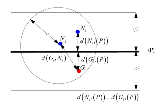
Рисунок 424: Призрачная частица, которая будет создана

Частицы, которые, как можно ожидать, будут оставаться далеко от плоскости симметрии на протяжении всего моделирования, никогда не будут симметризованы. Это дает возможность переоценить количество частиц, которые будут симметризованы за один момент.

Когда частица Ni должна быть симметризована относительно n условий, частица Ni порождает n призрачных частиц. Следующее количество должно оставаться меньше Maxsph (начиная с версии 14.0.220, “Maxsph” игнорируется, а память выделяется динамически).

\[\sum\nolimits_{n=1}^{n}n_{particles}\tag{311}\]

Где,

n Количество условий

\(n_{particles}\) Количество частиц, которые необходимо симметризировать относительно условия n

В любом случае, значение по умолчанию, которое является количеством условий симметрии SPH, умноженным на количество частиц, будет достаточно для решения любой проблемы.

Параметры преобразования твердого тела в SPH (Sol2SPH)

Параметр преобразования твердого тела в SPH (Sol2SPH) позволяет вам преобразовать твердый элемент в частицы, чтобы увеличить временной шаг/надежность расчета Лагранжа, не изменяя при этом физику.

Временной шаг

В PRADIOS доступны два метода временного шага SPH:

• Шаг времени частицы (/DT/SPHCEL)

• Узловой шаг времени (/DT/NODA)

В шаге времени частицы стабильный шаг времени вычисляется как:

\[\Delta t=\Delta T_{sca}\cdot\min\left(\frac{d_{i}}{c_{i}\left(\alpha_{i}+\sqrt{\alpha_{i}2+1}\right)}\right)\tag{312}\]

Где,

\(d_{i}\) Длина сглаживания, связанная с частицей

\(c_{i}\) Скорость звука в месте

\[\alpha_{i}=q_{a}+\frac{q_{a}\cdot\eta_{i}\cdot d_{i}}{c_{i}}\tag{313}\]

Для масштабного коэффициента шага времени \(\Delta T_{sca}\) рекомендуется установить его на 0,3.

В узловом временном шаге стабильный временной шаг вычисляется как:

\[\Delta t=\Delta T_{sca}\cdot\sqrt{\frac{2m}{K^{*}}}\tag{314}\]

Где,

m Масса для частиц

\(K^{*}\) Жесткость на основе взаимодействия SPH

Для масштабного коэффициента временного шага \(\Delta T_{sca}\) рекомендуется установить его равным 0,67.

Термический анализ

Теплопередача теперь доступна между частицами SPH и конечными элементами с \(I_{the}\) =1 в /INTER/TYPE7 и /INTER/TYPE21; и с /THERM_STRESS/MAT, тепловое расширение в SPH также возможно.

Опция Solid to SPH (Sol2SPH)

Опция Solid to SPH (Sol2SPH) позволяет превратить твердый элемент в частицы, чтобы увеличить временной шаг/надежность расчета Лагранжа, не изменяя при этом существенно физику.

Она совместима с опциями свойств твердого тела /PROP/TYPE14 (SOLID) и /PROP/TYPE6 (SOL_ORTH) и ограничена:

• \(I_{solid}\) = 1, 2 or 24

• \(I_{frame}\) = 1 or 2

• 8-узловые кирпичи (/BRICK включая вырожденные) и 4-узловые тетра (TETRA4), но не 10-узловые тетра.

Входные данные:

#---1----|----2----|----3----|----4----|----5----|----6----|----7----|----8----|----9----|---10----|
/PROP/SOLID/3
Пример реквизита
#  Isolid    Ismstr                Icpre  Itetra10     Inpts   Itetra4    Iframe                  dn
        1         2                    0         0         0         0         1                   0
#               q_a                  q_b                   h            LAMBDA_V                MU_V
                  0                    0                   0                   0                   0
#            dt_min    istrain      IHKT
                  0          0         0
#    Ndir  SPH_part
        1        10
#---1----|----2----|----3----|----4----|----5----|----6----|----7----|----8----|----9----|---10----|

SPH_часть

Номер детали, определяющий свойства SPH

Ndir

Nколичество частиц, созданных для каждого направления, максимальное значение — 9

Таблица 27: 8 узлов Brick

Частицы созданы в соответствии с кубической сеткой.

Таблица 28: 4 узла Tetra

Ndir = 1: 1 частица создана	Ndir = 2: 4 частиц создано	Ndir = 3: 10 частиц создано	Ndir = 4: 22 частиц создано

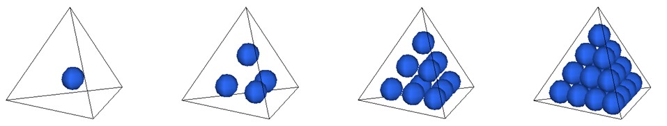
Переход от твердых элементов к частицам SPH может быть вызван контактом или удалением кирпича.

Поведение частиц Sol2SPH

Все частицы создаются в начале расчета.

Пока их основной элемент не удален, эти частицы неосвобождены.

Когда основной твердый элемент удален, частицы освобождаются и ведут себя как любая другая подлинная частица SPH.

Кинематика неосвобожденных частиц интерполируется из их основного элемента. В свою очередь, силы, приложенные к этим частицам, передаются в их соответствующие твердые узлы.

Эти силы:

• Контактные силы, если они вторичны по отношению к интерфейсу TYPE7 или жестким стенкам

• Силы взаимодействия с освобожденными частицами или подлинными частицами.

Процесс активации частиц

Частицы полностью активируются на основе следующих критериев.

• Их основной кирпич удаляется либо потому, что:

◦ Достигнут минимальный временной шаг (/DT/BRICK/DEL)

◦ Критерии отказа, связанные с законом о материалах кирпича, были выполнены

• В случае контакта:

◦ Если невыпущенная частица является вторичной по отношению к интерфейсу TYPE7 и

входит в зазор основной поверхности, кирпич удаляется, а связанные частицы освобождаются при условии, что флаг Ibag интерфейса установлен на 1.

◦ Если невыпущенная частица находится в пределах расстояния взаимодействия любой частицы, принадлежащей другой части (включая невыпущенные частицы), основной кирпич удаляется, а связанные частицы высвобождаются. Следовательно, между двумя частями Sol2SPH не требуется контактного интерфейса.

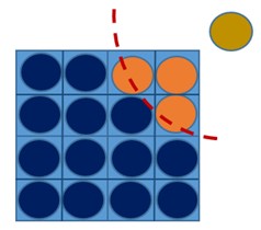
Рисунок 425: Оранжевые частицы высвобождаются, поскольку они находятся в пределах расстояния взаимодействия желтой частицы

(которая принадлежит другой части)

◦ Если Isol2sph установлен на 2 в /SPHGLO, то частицы не высвобождаются, если 2 части принадлежат к одному и тому же подмножеству. Эта опция может быть полезна для предотвращения нежелательной активации частиц на стыке частей, принадлежащих к одним и тем же физическим сущностям.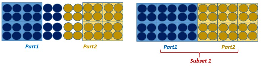

Рисунок 426: Isol2sph = 1: Нежелательная активация частиц / Isol2sph = 2 + определение подмножества

Свойства частиц определяются с помощью опции /PROP/SPH.

Типичное свойство для частиц Sol2SPH:

#---1----|----2----|----3----|----4----|----5----|----6----|----7----|----8----|----9----|---10----|
/PROP/TYPE34/10
SPH prop пример
#                 mp                  qa                  qb             alpha_cs  skew_ID      h_ID
                   0                   0                   0                    0        0         0
#    order                   h             xi_stab
         0               125.0                   0
#---1----|----2----|----3----|----4----|----5----|----6----|----7----|----8----|----9----|---10----|

Масса частиц автоматически пересчитывается из основного элемента для обеспечения сохранения массы. Для этого типа детали SPH входная масса может быть 0,0.

Длина сглаживания должна быть введена. Хорошее значение для регулярной сетки:

\[h=\frac{1.5\cdot l}{Ndir}\tag{315}\]

Где,

h Длина сглаживания

l Размер элементов кирпича

Ndir Количество частиц в каждом направлении для каждого твердого элемента

Материальный закон может быть /MAT/LAW2, /MAT/LAW3, /MAT/LAW4, /MAT/LAW6, /MAT/LAW12, /MAT/LAW21, /MAT/LAW24, /MAT/LAW36, /MAT/LAW49, or /MAT/LAW81.

Оба закона материала для твердого тела и SPH должны быть одного типа.

Параметры материала могут быть разными, но убедитесь, что они согласованы.

Рекомендуется сохранить те же параметры и изменить только значения отказа ( критерии отказа, максимальная деформация, давление откола, …).

Контакт между Sol2SPH и другими частями

Sol2SPH против части конечного элемента

Контакт должен быть определен через интерфейс TYPE7.

Часть Sol2SPH должна быть вторичной и должна быть тоньше, чем основная часть.

Контакт должен быть определен между основной (FE) частью и SPH частицами части Sol2SPH (номер детали определен, например, в SPH_PARTID).

Самоударяющиеся интерфейсы невозможны, но поскольку частицы взаимодействуют друг с другом, даже если они не активированы, самоконтакт части Sol2SPH всегда учитывается.

Коэффициенты жесткости и определение зазора следуют тем же правилам, что и обычные частицы SPH.

Частицы SOL2SPH могут быть автоматически активированы, а их соответствующий элемент кирпича удален при вводе расстояния зазора, если флаг \(I_{bag}\) интерфейса установлен на 1,0.

SOL2SPH против SPH или SOL2SPH

Контакт обрабатывается автоматически, и интерфейс не создается.

Другие руководства по моделированию

Ограничения

Sol2SPH несовместим с SPHBCS и параметрами входа/выхода.

Размеры ячеек и другие детали SPH

Все детали SPH и Sol2SPH должны иметь одинаковый шаг.

Поскольку конфигурация частиц Sol2SPH кубическая, детали SPH также должны использовать кубическую сетку.

/BRICK/DT/DEL

Использование /DT/BRICK/DEL является наиболее эффективным с точки зрения использования ЦП способом использования Sol2SPH.

Минимальный временной шаг должен быть примерно на 20-30% меньше естественного временного шага.

Рекомендуется использовать узловой временной шаг для лучшей стабильности частиц SPH.

После удаления блока шаг по времени может быть таким же низким, как:

\[\Delta t=\frac{\Delta T_{\text{min}}}{Ndir}\tag{316}\]

Где,

\(\Delta T_{\text{min}}\) Шаг по времени удаления блока, как определено в /DT/BRICK/DEL

Ndir Количество созданных частиц в каждом направлении

Многодоменная техника

Целью многодоменной техники (также называемой RAD2RAD) является оптимизация вычислительной производительности крупномасштабных моделей PRADIOS.

Целью многодоменной техники (также называемой RAD2RAD) является оптимизация вычислительной производительности крупномасштабных моделей PRADIOS, которые соответствуют определенным критериям:

• Возможность подразделить всю модель на ряд отдельных поддоменов с четко определенными интерфейсами/связями между ними.

• Различные поддомены должны характеризоваться разными размерами сетки и, следовательно, очень разными минимальными временными шагами.

Цель состоит в том, чтобы улучшить точность прогнозирования при разумном, возможно, выгодном времени вычисления для моделей с доменами с очень разными размерами временных шагов.

Например, привлекательно использовать многодоменную технику для вычисления больших моделей, которые имеют одну или несколько частей с мелкой сеткой для захвата определенных локальных явлений, таких как локализация/распространение трещин.

Еще более привлекательно использовать многодоменную технику для вычисления больших моделей взаимодействия жидкости и конструкции, как при моделировании приводнения или посадки самолета, где элементы жидкости с большими временными шагами многочисленны по сравнению с элементами структуры Лагранжа с очень малыми временными шагами.

В явной схеме интеграции, используемой решателем сбоев PRADIOS, шаг времени глобальной модели штрафуется элементами, имеющими наименьший шаг времени. Идея состоит в том, чтобы заменить эту глобальную модель физически эквивалентными поддоменами, разделяя части с различным минимальным шагом времени. Каждый поддомен разрешается как отдельная модель PRADIOS, использующая свой собственный шаг времени, передача силы и импульса между ними рассчитывается отдельной основной программой (RAD2RAD), гарантируя ограничения устойчивости.

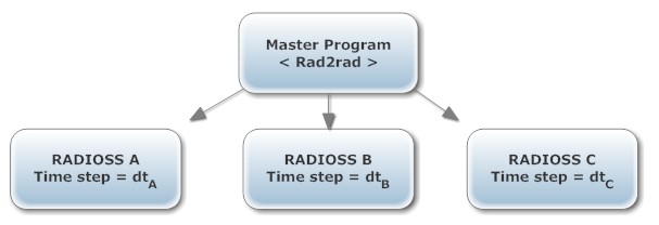
Рисунок 427:

Многодоменная эффективность основана на двух типах несоответствий:

• Размеры временных шагов

• Относительные размеры доменов

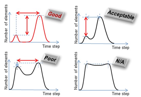
Рисунок 428:

Он особенно подходит для моделей с основными и поддоменами:

• очень разные плотности сетки, поэтому очень разные временные шаги

• разные формулировки, такие как Лагранж, ALE или Лагранж, и SPH, при условии, что область ALE или SPH больше области Лагранжа

Теоретическое ускорение

Эту эффективность многодоменного метода можно измерить с помощью коэффициента ускорения. Это отношение между затраченным временем исходного вычисления и затраченным временем, полученным с помощью многодоменного метода.

Если стоимость ЦП основной программы (RAD2RAD) и время, затраченное на коммуникации, незначительны, а временной шаг и стоимость за цикл каждого домена постоянны во время вычисления, можно вычислить оценку ускорения, чтобы определить, является ли использование многодоменного метода релевантным или нет.

В случае 2 доменов, A и B, где A является доменом с наименьшим временным шагом, ускорение можно получить с помощью следующей формулы:

\[Speedup=\frac{T_{MONO}}{T_{MULTI}}=\frac{\big{(}Ne_{A}C_{A}+Ne_{B}C_{B}\big{)}Nc_{A}}{Ne_{A}C_{A}Nc_{A}+Ne_{B}C_{B}Nc_{B}}\tag{317}\]

Где,

Nc Количество циклов для каждого домена

Ne Количество элементов каждого домена

3. Средняя стоимость на элемент и на цикл для каждого домена

Формулу можно переписать так:

\[Speedup=\frac{\zeta+(1-\zeta)\cdot\psi}{\zeta\cdot\gamma+(1-\zeta\cdot\gamma)\cdot\psi}\tag{318}\]

Где,

\(\zeta=\frac{C_{A}}{C_{B}}\) Среднее соотношение стоимости за цикл между доменами

\(\gamma=\frac{Nc_{A}}{Nc_{B}}=\frac{dt_{B}}{dt_{A}}\) Соотношение временных шагов

\(\psi=\frac{Ne_{A}}{Ne_{A}+Ne_{B}}\) Процент элементов в домене с наименьшим временным шагом

Если средняя стоимость за цикл одинакова в двух доменах, то формула становится:

\[Speedup=\frac{1}{\gamma+(1-\gamma)\cdot\psi}\tag{319}\]

Таким образом, ускорение очень велико, когда \(\gamma\) и \(\psi\) близки к нулю, что означает, что область A мала по сравнению с B, а отношение временного шага велико. Это то, что изображено на Рисунок 428.

Настройка модели

Две возможные настройки модели: - Формат файла с одним входом

• Формат файла с несколькими входами

Прогоны PRADIOS полностью независимы и не взаимодействуют напрямую друг с другом. Каждый поддомен использует свой собственный временной шаг, как описано ниже:

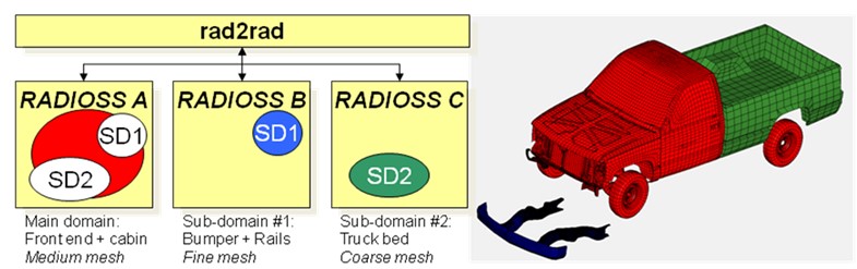
Рисунок 429:

Временной шаг каждого поддомена произволен; но для достижения наилучшего прироста в плане ускорения они должны значительно отличаться друг от друга.

Наилучшая ручная декомпозиция будет получена путем разделения глобальной модели на части с большим количеством элементов, имеющих большой временной шаг с одной стороны, и небольшим количеством элементов с малым временным шагом с другой стороны.

Все коммуникации, передача данных, синхронизация временного шага, условия равновесия и устойчивости на границах домена обеспечиваются основной программой.

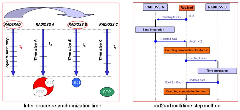
Рисунок 430:

Новое в 14.0

Начиная с 14.0, возможно моделирование взаимодействия жидкости и конструкции, включая ALE и/или SPH.

Новое в 13.0

Начиная с 13.0, Multi-Domain полностью совместим с Hybrid-MPP, т. е. позволяет многопоточность для RAD2RAD.

Подсказки

Для лучшей вычислительной производительности:

• Поддомен должен составлять менее 30% от полного домена (основной _ поддомены) с точки зрения узлов или элементов, а естественное (или приемлемое масштабирование массы) отношение временного шага между поддоменом и основными доменами должно быть ниже 1/3.

• Применить то же правило для чистых моделей Лагранжа или FSI, которое заключается в том, чтобы поместить части со значительно меньшим временным шагом в поддомен.

• Для чистых моделей Лагранжа Multi-Domain рабочая нагрузка RAD2RAD должна быть максимально минимизирована путем сокращения потока связи между доменами, с этой целью интерфейсы контактов и соединения между поддоменами и основными доменами должны быть максимально минимизированы.

• Важно проверить, что поддомен не является частью глобального интерфейса контакта, но имеет свой собственный поддоменный самовоздействие, и создать междоменные контакты не больше, чем необходимо.

• Настоятельно рекомендуется симметризировать каждый созданный междоменный контактный интерфейс.

• Для многодоменных систем с ALE или SPH нет необходимости минимизировать контактные интерфейсы между жидкостью и конструкцией.

• Для моделей с поддоменом, имеющим относительно небольшое количество элементов, количество выделенных ЦП должно соответствовать эмпирическому правилу не менее 2000 элементов на ЦП, и рекомендуется использовать максимально возможное количество потоков на узел используемого кластера.

• В одной модели разрозненные части с низкими временными шагами не обязательно оправдывают несколько поддоменов. Если эти части имеют схожие низкие временные шаги, их необходимо поместить в один поддомен.

• Если соединения между поддоменами и основными доменами также имеют небольшой временной шаг, эти соединения должны быть частью поддомена.

• Поддомены, в основном состоящие из трехмерных элементов Лагранжа, делают многодоменный режим менее эффективным, чем если бы он состоял из двухмерных и одномерных элементов.

• Для многодоменного FSI рекомендуется использовать жидкость в главном домене и определять /DT/ALE с элементарным свободным временным шагом с коэффициентом масштабирования 0,5 для ALE. В поддомене Лангранжа следует использовать узловой временной шаг /DT/NODA с коэффициентом масштабирования 0,9.

Формат единого входного файла

Настройка модели

Настройка формата множественного ввода была впервые представлена ​​в PRADIOS Мультидоменной технике. Главным недостатком этой настройки является то, что она предполагает много работы для пользователя, который должен вручную создавать несколько независимых входных файлов. Это может быть очень долго, сложно и источником ошибок в случае небольших доменов, извлеченных из очень больших и сложных моделей.

Цель настройки одного входного файла - упростить задачу пользователя путем автоматического создания поддоменов. Требуется только один входной файл Starter, который включает всю модель, как классическое вычисление. Необходимо указать только части модели для размещения в поддоменах. Затем Starter автоматически извлекает указанные домены из полной модели и генерирует один файл перезапуска для каждого домена. При использовании этого метода может быть только один поддомен, но этот поддомен может состоять из нескольких частей.

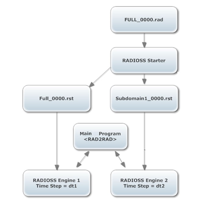
Fрисунок 431: Архитектура настройки поддомена

В настоящее время можно указать только один домен, но это ограничение может быть расширено в будущем.

Автоматическое создание поддомена

Поддомен просто определяется списком частей.

Модель разделения

Первый шаг создания поддомена — разделение полной модели. Это достигается путем запуска одного дочернего процесса Starter на домен. Каждый процесс сохраняет только часть, связанную с ним, и соответствующие узлы и элементы. Группы сущностей, такие как /GRNOD, /GRPART или /SURF, также разделяются, что позволяет разделить множество опций (если опция ни на что не ссылается в одном домене, она подавляется). Некоторые опции сложнее разделить и требуют особой обработки, которая часто подразумевает изменение определения домена. Некоторые другие опции не могут быть разделены. Для получения дополнительной информации о опциях, несовместимых с Multi-Domains, см. Текущие ограничения. В результате поддомен большую часть времени состоит из частей, указанных пользователем (с их связанными узлами и элементами), а также некоторых других элементов или узлов, которые автоматически добавляются из-за разделения некоторых опций.

Связи между доменами

Вторым шагом является обнаружение взаимодействий между доменами. Первый тип взаимодействия — это прямое соединение. Starter автоматически обнаруживает общие узлы между доменами и создает соединения Node-to-Node.

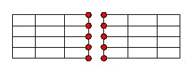
Рисунок 432:

Контакт между доменами

Второй тип взаимодействия между доменами — это контакт. Вычисление контактных сил между доменами основано на методе искусственной кожи. Это означает, что контакты не вычисляются внешней программой RAD2RAD, а внутри одного из двух доменов, называемых основным доменом.

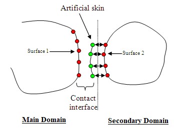
Рисунок 433:

При настройке одного входного файла контакты между доменами всегда вычисляются в поддомене, в основном потому, что качество связи гораздо лучше, когда контакт обрабатывается в домене с наименьшим шагом по времени.

Поэтому поверхности основного домена, затронутые контактом с поддоменом, автоматически дублируются в этом поддомене с пустым материалом, имеющим ту же плотность и модуль Юнга. Затем устанавливается междоменная связь узел-узел между узлами искусственной кожи в поддомене и узлами исходной поверхности в основном домене.

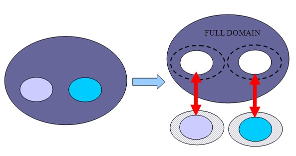
Рисунок 434:

Это означает, что для получения хороших характеристик все контакты между основным и поддоменом должны быть помещены в определенные контактные интерфейсы с как можно меньшими контактными поверхностями, но без пропуска потенциальных контактов. Например, если в модели с одним поддоменом используется только один самоконтактный интерфейс, поддоменом может потенциально влиять на все части основного домена, тогда основной домен будет полностью дублирован с пустым материалом внутри поддомена. Стоимость RAD2RAD будет огромной, а характеристики очень низкими.

Примечание: Если интерфейсы контактов определены плохо, выдается предупреждающее сообщение мультидоменный интерфейс слишком большой, если размер дублированной части меньше 50% от размера полной модели. Если этот процент больше 50%, выдается сообщение об ошибке.

Кроме того, настоятельно рекомендуется не иметь асимметрично определенных кросс-доменных контактных интерфейсов, где поддомен определен только на вторичной или основной стороне интерфейса. В этом случае только часть контактного интерфейса вычисляется в поддомене, то, что остается, вычисляется в основном домене. Чтобы избежать асимметричных контактных интерфейсов, рекомендуется систематически симметризировать кросс-доменные контактные интерфейсы (путем определения поддомена на обеих: основной и вторичной сторонах кросс-доменного контакта или исправления уже существующих асимметричных контактов путем добавления симметричного контактного интерфейса).

Примечание: Если интерфейс контакта между доменами разделен, выдается предупреждающее сообщение интерфейс контакта между доменами разделен.

Контактные интерфейсы PRADIOS, совместимые с Multi-Domain:

• /INTER/TYPE5

• /INTER/TYPE7

• /INTER/TYPE11

• /INTER/TYPE18

• /INTER/TYPE24, if (surf_ID₁ > 0, surf_ID₂ > 0) or (surf_ID₁ > 0, surf_ID₂ = 0). Not if (grnd_IDs > 0, surf_ID₁= 0, surf_ID₂ >0).

Пользовательские соединения между доменами

Некоторые кинематические условия также могут создавать соединения между доменами, если они определены через интерфейс Multi-Domains.

• Твердые тела: в случае твердых тел, соединяющих два домена, применяется особая обработка. Твердое тело разделяется на два, и для каждого домена выполняется вычисление массы, матрицы инерции и положения центра тяжести. Затем два основных узла двух частей твердого тела связываются с помощью RAD2RAD с использованием формулировки, аналогичной той, которая используется для классической связи узел-узел, но адаптированной к несферической инерции.

• Связанный интерфейс: в случае связанного интерфейса TYPE2 с основными элементами в одном домене и вторичными узлами в другом, используется другая стратегия. Эта стратегия похожа на ту, что применяется для контактов. Основные элементы дублируются с помощью пустотного материала в домене, содержащем вторичные узлы, чтобы полностью определить связанный интерфейс в этом домене. Затем многодоменная связь применяется только к узлам основных элементов. Если оба домена содержат вторичные узлы, дублирование основных элементов выполняется с обеих сторон.

• Жесткие связи, RBE3 и цилиндрические соединения: та же идея применяется к жесткой связи и RBE3. Если один из этих вариантов имеет вторичные узлы на двух доменах, все отсутствующие вторичные узлы дублируются с обеих сторон, и все вторичные узлы соединяются RAD2RAD. Затем этот вариант вычисляется с обеих сторон.

Другие типы соединений не могут быть разделены. Это означает, что эти соединения могут использоваться только внутри одного домена и вне зоны соединения. Этими вариантами являются:

• /MPC

• /RBE2

• /GJOINT

Ввод данных

Вводной файл для стартера

Поддомены указываются по частям.

/SUBDOMAIN/subdomain_ID
subdomain_title
Part 1   Part 2   ...   Part n

Где,

Часть

Идентификатор частей, которые принадлежат поддомену

subdomain_ID

Идентификатор домена

subdomain_title

Имя поддомена (которое будет корневым именем одного файла движка)

Входной файл движка

Для каждого домена требуется один входной файл Engine, и для активации связи эти файлы должны содержать следующую директиву:

/RAD2RAD/ON

Одно имя файла Engine взято из rootname входного файла Starter: "full_model_rootname"_0001.rad, а другое имя входного файла Engine, относящегося к поддомену, взято из subdomain_title: subdomain_title_0001.rad, заданного для карты /SUBDOMAIN во входном файле Starter.

Входной файл RAD2RAD

Входной файл RAD2RAD — это текстовый файл, определяющий некоторую дополнительную информацию, требуемую программой RAD2RAD. При настройке поддомена входной файл RAD2RAD автоматически генерируется Starter. К нему можно получить доступ и изменить его, чтобы изменить параметры вычисления Multi-Domain перед запуском процессов RAD2RAD и Engine. Имя этого файла основано на полном корневом имени модели “_model_rootname”_0000.r2r.

Вывод данных

Файлы вывода Starter

Отдельные файлы вывода Starter генерируются для каждого домена.

Файлы истории времени

Создается один файл истории времени, содержащий всю информацию из обоих доменов. Этот файл имеет то же корневое имя, что и входной файл Starter. Содержимое этого файла эквивалентно тому, что получается после классического вычисления монодомена.

Все параметры для вывода истории времени (тип истории времени, частота вывода, формат и т. д.) должны быть указаны в файле Engine основного домена. Если параметры для истории времени определены во входном файле Engine поддомена, они будут проигнорированы.

Поскольку частота распечатки файла TH определяется основным доменом, минимальный временной интервал, разрешенный между двумя распечатками файла TH, является временным шагом основного домена. Для большей точности рекомендуется использовать временную частоту, которая намного выше временного шага основного домена.

Файлы ABF

Каждый PRADIOS Engine генерирует один файл ABF. Поэтому для построения всех глобальных переменных модели необходимо суммировать глобальные переменные каждого домена.

Выходной файл

Глобальные переменные всей модели можно вычислить, просто суммируя глобальные переменные, напечатанные в выходном файле каждого домена (каждый выход Engine).

Есть два исключения:

• Ошибка энергии: энергетический баланс вычисляется в каждом домене независимо от другого домена. Это означает, что для каждого домена силы связи Multi-Domain считаются внешними силами, и их работа добавляется к работе внешних сил. Эта работа используется только внутренне для вычисления энергетического баланса. Она не включается в значение работы внешних сил, напечатанное в выходном файле или в истории времени.

• Изменение массы: изменение массы также вычисляется локально, то есть это отношение добавленной массы в выбранном домене к массе этого домена.

Файлы анимации

Набор файлов анимации генерируется каждым движком. С помощью HyperView можно визуализировать два домена одновременно, просто сделав наложение.

Выходной файл RAD2RAD

Выходной файл rad2rad.out генерируется исполняемым файлом RAD2RAD. Этот файл содержит полезную информацию о связях между доменами (количество общих узлов, тип связи и т. д.).

Оценка SPEEDUP

Начиная с версии 14.0, оценка ускорения вычисляется в Starter, чтобы определить потенциальную эффективность многодоменного метода. Значение печатается в выходном файле Starter основного домена. Таким образом, если во время вычисления временные шаги резко меняются в одном домене, оценка ускорения будет неактуальной.

Параметры управления временным шагом, определенные во входном файле Engine (/DT/NODA/CST, /DTIX, …), учитываются в оценках временного шага в Starter.

Выделение ЦП

Домены PRADIOS обрабатываются последовательно, что означает, что одновременно запускается только один процесс PRADIOS. Общий ресурс ЦП автоматически выделяется работающему процессу, а остальные переводятся в режим ожидания без потребления ЦП. При настройке поддомена одинаковое количество доменов SPMD автоматически выделяется всем доменам. Для лучшей производительности для каждого домена при работе в Hybrid-MPP следует использовать одинаковое количество потоков SMP на домен SPMD.

Начиная с версии 12.0.210 исполняемый файл RAD2RAD полностью распараллелен. Это означает, что RAD2RAD должен быть запущен точно так же, как исполняемые файлы Engine (те же параметры mpi) и что для процессов Engine и RAD2RAD должно использоваться одинаковое количество доменов SPMD.

Запуск многодоменного анализа

Существует два способа запуска многодоменных вычислений: с помощью Laduga Compute Console или вручную.

1. Самый простой способ запуска многодоменных вычислений — использовать Laduga Compute Console.

1. Выберите файл Multi-Domain Starter в качестве входного файла и определите количество ядер, которые будут использоваться в моделировании.

   Затем Compute Console запустит Starter, Engine и процесс RAD2RAD. Подробнее об использовании Laduga Compute Console с PRADIOS см. в Laduga Compute Console (ACC).

2. Чтобы запустить многодоменное вычисление, используйте командную строку для перехода в рабочий каталог, содержащий входные файлы.

3. Запустите Starter в терминале с помощью команды:

   Option

   Description

   Linux

   <install_dir>/hwsolvers/bin/linux64/starter_version -i "rootname"_0000.rad

   Windows

   <install_d ir>\\hwsolvers\\bin\\win64\\starter_version -i "rootname"_0000.rad

4. Запустите RAD2RAD в терминале с помощью команды:

   OptionL

   Description

   Linux

   <install_dir>/hwsolvers/bin/linux64/r2r_version “rootname”_0000.r2r

   Windows

   <install_dir>\hwsolvers\bin\win64\r2r_version “rootname”_0000.r2r

Затем RAD2RAD будет ожидать подключений PRADIOS от отдельных

доменов.

Примечание: Файл "rootname"_0000.r2r автоматически создается Starter.

5. Запустите движок для каждого домена в отдельных терминалах.

   Параметр

   Описание

   Linux

   <install_dir>/hwsolvers/bin/linux64/engine_version -i “rootname”_0001.rad

   Windows

   <install_dir>\hwsolvers\bin\win64\engine_version -i rootname_of_the_subdomain”_0001.rad

Все процессы PRADIOS затем автоматически подключатся к RAD2RAD.

6. Запустите ручной скрипт SMP.

Linux : run_linux_SMD
./s_<version>_linux64 -i FULL_0000.rad
./e_<version>_linux64 -nt 4 -i FULL_0001.rad > out_1 &
./e_<version>_linux64 -nt 4 -i SUBDOM_0001.rad > out_2 &
./r2r_<version>_linux64 -nt 4 FULL_0000.r2r

Windows : run_win_SMD.bat
E:\\Rad2rad\\s_<version>_win64.exe -i FULL_0000.rad
set KMP_STACKSIZE=64M
start /B E:\\Rad2rad\\e_<version>_win64.exe -nt 4 -i FULL_0001.rad > out1
start /B E:\\Rad2rad\\e_<version>_win64.exe -nt 4 -i SUBDOM_0001.rad > out2
start /B E:\\Rad2rad\\r2r_<version>_win64.exe -nt 4 FULL_0000.r2r

Windows (cygwin) : run_win_SMD
./s_<version>_win64.exe -i FULL_0000.rad;
./e_<version>_win64.exe -nt 4 -i FULL_0001.rad > out1&
./e_<version>_win64.exe -nt 4 -i SUBDOM_0001.rad > out2&
./r2r_<version>_win64.exe -nt 4 FULL_0000.r2r;

7. Запустите ручной скрипт SPMD.

Linux : run_linux_SPMD
./s_<version>_linux64 -np 4 -i FULL_0000.rad
mpiexec -n 4 ./e_<version>_linux64_impi -i FULL_0001.rad > out_1 &
mpiexec -n 4 ./e_<version>_linux64_impi -i SUBDOM_0001.rad > out_2 &
mpiexec -n 4 ./r2r_<version>_linux64_impi FULL_0000.r2r

Windows : run_win_SPMD.bat
E:\\Rad2rad\\s_12_main_win64.exe -np 4 -i FULL_0000.rad
set KMP_STACKSIZE=64M
start /B mpiexec -n 4 E:\\Rad2rad\\e_<version>_win64_impi.exe -i FULL_0001.rad> out1
start /B mpiexec -n 4 E:\\Rad2rad\\e_<version>_win64_impi.exe -i SUBDOM_0001.rad> out2
start /B mpiexec -n 4 E:\\Rad2rad\\r2r_<version>_win64_impi.exe FULL_0000.r2r

Windows (cygwin) : run_win_SPMD
./s_<version>_win64.exe -np 4 -i FULL_0000.rad;
mpiexec -n 4 ./e_<version>_win64_impi.exe -i FULL_0001.rad > out1&
mpiexec -n 4 ./e_<version>_win64 impi.exe -i SUBDOM_0001.rad > out2&
mpiexec -n 4 ./r2r_<version>_win64 impi.exe FULL_0000.r2r;

Текущие ограничения

Можно определить только один поддомен.

Эти параметры несовместимы с /SUBDOMAIN:

• /DFS/DETPOINT/NODE

• /FX_BODY

• /SPHBCS

Следующие соединения могут использоваться только внутри одного домена, но не могут использоваться в зоне сопряжения или через многодоменный интерфейс.

• /GJOINT

• /MPC

• /RBE2

Multi-Domain несовместим со всеми кинематическими условиями, основанными на множителях Лагранжа, из-за несовместимости с формулировкой связи.

Multi-Domain пока несовместим с AMS (Advanced Mass Scaling), Reyleigh Damping (/DAMP), Dynamic Relaxation (/DYREL), если только узлы не являются частью кросс-доменного интерфейса или контакта, интерфейсы TYPE1.

Датчики типа GAUGE, INTER и RWAL еще не синхронизированы между доменами. Это означает, что если датчик и все его связанные функции не ограничены одним доменом, поведение этого датчика может быть неправильным. Тем не менее, датчики типа DIST, ACCE и TIME полностью совместимы с Multi-Domain и синхронизированы между доменами.

Настройка модели

Настройка формата множественного ввода была первой, введенной в технике PRADIOS Multi-Domain. Каждый поддомен строится как отдельная полная модель PRADIOS, использующая собственные полные входные файлы. Связь между вычислениями PRADIOS Engine обеспечивается программой RAD2RAD на основе связей между доменами, определенными в каждой модели PRADIOS.

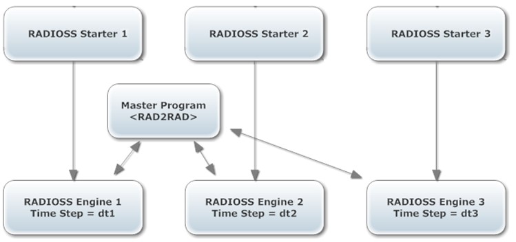
Рисунок 435:

Соединение между доменами

Соединение (или связь) между 2 доменами всегда определяется 2 группами узлов, относящихся к двум соответствующим сеткам, которые должны быть соединены друг с другом, и типом этого соединения. Ниже приведен список доступных типов соединений в RAD2RAD.

ТИП 1: Оболочка к оболочке (двойной метод Шура)

Его можно использовать для связи сеток элементов оболочки через множители Лагранжа. Сетки могут быть совместимыми или несовместимыми, а интерфейсы могут быть открытыми или закрытыми.

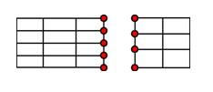
Рисунок 436:

Примечание: В случае несовместимых сеток и открытого интерфейса начальная и конечная точки двух граней должны совпадать. В том же направлении, в случае закрытого интерфейса, должна быть хотя бы одна общая точка между двумя гранями.

TYPE 2: Оболочка к балке (двойной метод Шура)

Этот тип связи очень похож на ТИП 1; но он адаптирован для соединения балка/оболочка.

Примечание: Ограничения на оболочку те же что и для ТИПА 1 в случае несовместимых сеток.

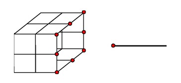
Рисунок 437:

ТИП 4: Узел к узлу (метод Шура Primal)

В случае совместимых сеток связь между доменами можно свести к простым отношениям узел к узлу.

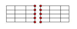
Рисунок 438:

Этот метод строго эквивалентен ТИПУ 1 для совместимых сеток; но потребляет меньше процессорного времени, поскольку не требуется выполнять сборку матрицы и инверсию. Кроме того, в этом случае, поскольку требуются только узловые данные, его можно использовать для соединения узлов любого типа (прикрепленных к любому типу элементов).

Примечание: В случае соединения оболочки с твердым телом условие непрерывности применяется только к поступательной степени свободы.

Контакт между доменами

ТИП 5: Соединение

Также возможно вычислить контакт между доменами с помощью метода искусственной кожи. Контакты не вычисляются RAD2RAD, а внутри одного из двух доменов, называемых основным доменом. Поэтому часть вторичного домена, затронутая контактом, должна быть продублирована в основном домене с пустотным материалом, имеющим ту же плотность и модуль Юнга. Затем контакт обрабатывается PRADIOS как обычно внутри основного домена, и для соединения узлов искусственной кожи и соответствующих узлов вторичного домена должно использоваться соединение типа 5, специфичное для узла (похожее на соединение типа 4).

Рисунок 439:

В главном входном файле Multi-Domain определение соединения TYPE5 аналогично другим соединениям; за исключением того, что узлы основного домена (узлы искусственной кожи) должны быть объявлены первыми:

/LINK/TYPE5
Main_Domain Link_Id1
Second_Domain Link_Id2

Контактные интерфейсы PRADIOS, совместимые с Multi-Domain:

• /INTER/TYPE5

• /INTER/TYPE7

• /INTER/TYPE10

• /INTER/TYPE11

• /INTER/TYPE18

• /INTER/TYPE24, if (surf_ID₁1 > 0, surf_ID₂ > 1) or (surf_ID₁ > 0, surf_ID₂ = 0). Not if (grnd_IDs > 0, surf_ID₁ = 0, surf_ID₂ > 0).

Примечание: Соединение RAD2RAD TYPE5 несовместимо с контактными интерфейсами, использующими формулировку множителей Лагранжа. Масса и узловая жесткость переносятся соединением RAD2RAD TYPE5 из вторичного домена в искусственную кожу. Поэтому изменения массового и узлового временного шага могут наблюдаться в основном домене в начале вычисления.

В главном входном файле Multi-Domain определение соединения TYPE5 аналогично другим соединениям; за исключением того, что узлы основного домена (то есть узлы искусственной оболочки) должны быть объявлены первыми:

/LINK/TYPE5
Main_Domain Link_Id1
Second_Domain Link_Id2

Если кинематические ограничения применяются к части вторичной области, которая дублируется в основной области, они должны дублироваться в случае:

• A rigid body duplication, the main node must be specified in the RAD2RAD connection TYPE5.

• Interface TYPE2 duplication, an additional flag /TIED must be specified in the RAD2RAD input file.

Примечание: Для твердых тел или интерфейсов TYPE2 вторичные узлы можно удалить из соединения RAD2RAD. Их поведение определяется только их основными узлами или основными элементами. Поэтому Multi-Domains не будет оказывать на них никакого влияния. RAD2RAD несовместим с кинематическими условиями множителей Лагранжа, такими как интерфейс /INTER/LAGMUL/TYPE2 and /RWALL/LAGMUL.

Ввод данных

Файл ввода для стартера

Определение соединений (или ссылок) между доменами:

/EXTERN/LINK/Link_ID title gr_ID

Где,

gr_ID

Идентификатор узловой группы, определяющий пограничные узлы с другими доменами

Link_ID

Идентификатор ссылки

Количество внешних ссылок в модели PRADIOS не ограничено. Единственное ограничение заключается в том, что разные ссылки не должны содержать общие узлы. Каждая ссылка определяет отдельный интерфейс между текущей моделью и внешним миром.

Входной файл Engine

Для каждого домена требуется один входной файл Engine. Чтобы активировать связь, все файлы Engine должны содержать следующую директиву:

/RAD2RAD/ON

Входной файл RAD2RAD — это текстовый файл, определяющий некоторую дополнительную информацию, требуемую программой RAD2RAD. Имена доменов для подключения и соединения между доменами должны быть указаны во входном файле RAD2RAD. Для каждого соединения должны быть указаны идентификаторы соединенных ссылок и используемые типы соединений. Также должны быть введены некоторые специфичные для Multi-Domain параметры.

Примечание: Для получения дополнительной информации о входном файле RAD2RAD обратитесь к онлайн-документации Multi-Domain.

Выделение ЦПУ

Домены PRADIOS обрабатываются поочередно; это означает, что только один процесс PRADIOS работает одновременно. Полный ресурс ЦП автоматически выделяется RAD2RAD работающему процессу Engine, а остальные процессы переводятся в режим ожидания без потребления ЦП. Это означает, что все доступные ресурсы ЦП должны быть выделены каждому домену во время его вычисления.

Запуск многодоменного анализа

Существует два способа запуска многодоменного вычисления: вручную и через скрипт.

Пример скрипта SMP

Пример скрипта SPMD

1. Чтобы вручную запустить многодоменное вычисление, используйте командную строку для перехода в рабочий каталог, содержащий входные файлы отдельных доменов (_0000.rad и _0001.rad) и главный входной файл многодоменного вычисления (input.dat).

2. Запустите Starter для каждого домена в терминале с помощью команды:

   Option

   Description

   Linux

   <install_dir>/hwsolvers/bin/linux64/s_version-i "filename"

   Windows

   <install_dir>\\hwsolvers\\bin\\win64\\s_version -i "filename"

3. Запустите RAD2RAD в терминале с помощью команды:

   Option

   Description

   Linux

   <install_dir>/hwsolvers/bin/linux64/r2r_version input.dat

   Option

   Description

   Windows

   <install_dir>\\hwsolvers\\bin\\win64\\r2r_version input.dat

Затем RAD2RAD будет ожидать подключений PRADIOS от отдельных доменов.

4. Запустите движок для отдельных доменов в отдельных терминалах, как показано ниже:

   Вариант

   Описание

   Linux

   <install_dir>/hwsolvers/bin/linux64/e_version -i "filename"

   Windows

   <install_dir>\\hwsolvers\\bin\\win64\\e_version -i "filename"

Все процессы PRADIOS затем автоматически подключатся к RAD2RAD.

Более простой способ запустить многодоменное вычисление — использовать скрипт.

5. Запустите Starter для каждого домена так же, как описано выше.

6. Добавьте скрипт с именем run_SMP или run_SPMD в свой рабочий каталог.

7. В скрипте измените имя входных файлов, расположение исполняемых файлов (MPI, RAD2RAD и PRADIOS Engine) и количество процессоров, если необходимо.

8. Запустите скрипт в терминале. Пример SMP

Linux : run_linux_SMP
./s_<versin> < PART1_0000.rad
./s_<version> < PART2_0000.rad
./e_<version> < PART1_0001.rad > out_1 &
./e_<version> < PART2_0001.rad > out_2 &
./r2r_<version> input.dat

Windows : run_win_SMP.bat
E:\\Rad2rad\\s_<version>.exe -i PART1_0000.rad
E:\\Rad2rad\\s_<version>.exe -i PART2_0000.rad
set KMP_STACKSIZE=64M
start /B E:\\Rad2rad\\e_<version>.exe -i PART1_0001.rad > out1
start /B E:\\Rad2rad\\e_<version>.exe -i PART2_0001.rad > out2
start /B E:\\Rad2rad\\r2r_<version>.exe input.dat

Windows (cygwin) : run_win_SMP
./s_<version>.exe < PART1_0000.rad; ./s_<version>.exe < PART2_0000.rad;
./e_<version>.exe < PART1_0001.rad > out1&
./e_<version>.exe < PART2_0001.rad > out2&
./r2r_<version>.exe data4.dat;

SPMD Example

Linux : run_linux_SPMD
./s_<version> < PART1_0000.rad
./s_<version> < PART2_0000.rad
/opt/hpmpi/bin/mpirun -np 4 ./e_<version> < PART1_0001.rad > out_1 &
/opt/hpmpi/bin/mpirun -np 4 ./e_<version> < PART2_0001.rad > out_2 &
../exec/r2r_<version>_impi data4.dat

Windows : run_win_SPMD.bat
E:\\Rad2rad\\s_<version>.exe -i PART1_0000.rad -n 4
E:\\Rad2rad\\s_<version>.exe -i PART2_0000.rad -n 4
set KMP_STACKSIZE=64M
start /B mpiexec -n 4 E:\\Rad2rad\\e_<version>.exe -i PART1_0001.rad > out1
start /B mpiexec -n 4 E:\\Rad2rad\\e_<version>.exe -i PART2_0001.rad > out2
start /B E:\\Rad2rad\\r2r_<version>.exe input.dat

Windows (cygwin) : run_win_SPMD
./s_<version>.exe < PART1_0000.rad;
./s_<version>.exe < PART2_0000.rad;
mpiexec -n 4 ./e_<version>.exe < PART1_0001.rad > out1&
mpiexec -n 4 ./e_<version>.exe < PART2_0001.rad > out2&
./r2r_<version>.exe data4.dat;

Распараллеливание RAD2RAD

Если размеры интерфейсов Multi-Domain велики, время, затрачиваемое в RAD2RAD на вычисление сил сцепления, может быть большим. Теперь можно сократить это время, разделив задачу вычисления сцепления между несколькими процессорами. В отличие от настройки одного входного файла, для настройки нескольких входных файлов доступна только SMP-распараллеливание RAD2RAD. Количество процессоров, которые могут быть использованы, должно быть меньше, чем количество ядер, доступных на аппаратном узле, где запущен RAD2RAD. Например, хорошее значение - 6 для машины с 8 ядрами. Количество потоков для RAD2RAD можно указать с помощью -nt в командной строке, как для Engines, или непосредственно во входном файле RAD2RAD с помощью ключевого слова /PROC/nthread. +———————————————————————–+ | Примечание: Влияние распараллеливания RAD2RAD | | на время ЦП незначительно, если количество узлов, обрабатываемых | | | | RAD2RAD, невелико ( < Nb of Cpus x 1000). | +———————————————————————–+

Примечание: Поскольку подключенные PRADIOS Engines находятся в спящем режиме когда RAD2RAD активен, параллелизация RAD2RAD когда RAD2RAD активен, параллелизация RAD2RAD не зависит от параллелизации Engines. Это означает, что одинпроцессор может быть назначен всем Engines, а также один процессор назначен RAD2RAD. Они будут использовать его один за другим.

MPI Настройки

При использовании исполняемых файлов Multi-Domains и SPMD Engine для улучшения производительности следует использовать следующие переменные среды MPI:

• HP-MPI: MPI_FLAGS set to y0

• Open-MPI: OMPI_MCA_mpi_yield_when_idle установлено значение 1

• Intel-MPI: можно использовать настройки по умолчанию

Выходные файлы

• PRADIOS: Отдельные выходные файлы генерируются каждым процессом PRADIOS.

• RAD2RAD: RAD2RAD генерирует определенный выходной файл с именем rad2rad.out.

Ограничения версии

• Каждый поддомен создается как завершенный. Отдельная модель PRADIOS, использующая собственные полные входные файлы.

• Передача данных между процессами PRADIOS и основной программой использует метод канальной системы связи. Все движки PRADIOS и RAD2RAD должны быть запущены на одном аппаратном узле.

• Кинематические условия на общих узлах между доменами совместимы только с соединением TYPE5.

• Программа RAD2RAD не распараллеливается для настройки нескольких входных файлов. Это может привести к снижению производительности в многодоменных вычислениях с большими поддоменами, работающими на большом количестве ЦП.

• В настоящее время многодоменное исчисление не выполняется автоматически основной программой. Все стартеры PRADIOS должны быть выполнены до запуска программы RAD2RAD. Хотя пакетное выполнение возможно, RAD2RAD и все процессы движка PRADIOS должны быть запущены независимо и параллельно на одном аппаратном узле.

• Для каждого домена PRADIOS количество ссылок ограничено 15, а количество ЦП ограничено 128.

Пример: Входной файл RAD2RAD

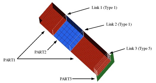
Рисунок 440: Модель

Входной файл RAD2RAD

$===============================================================
$ RAD2RAD R8 ВХОДНОЙ ФАЙЛ:
$======================================================================
$ 1. ОПРЕДЕЛЕНИЕ ДЕТАЛЕЙ
$=========================================================================
/ДОМЕН/ЧАСТЬ3 9
$=====================================================================
$ 2. ОПРЕДЕЛЕНИЕ ИНТЕРФЕЙСОВ
$===============================================================
/LINK/TYPE1 ЧАСТЬ1 2
ЧАСТЬ2 5
/ССЫЛКА/ТИП1
ЧАСТЬ1 1ЧАСТЬ2 4
/ССЫЛКА/ТИП5 ЧАСТЬ3 9
ЧАСТЬ1 3
$===========================================================================
$3 ВАРИАНТЫ
$=========================================================================
/MLTPS/ON 0.1 0.1 /СЕТКА/МОРФИН /РАДИУС/1e-7
/КОНЕЦ $========================================================================

Оптимизация дизайна

Оптимизация в PRADIOS была введена в версии 13.0. Она реализуется путем вызова возможностей оптимизации OptiStruct и одновременного использования решателя PRADIOS для анализа.

Оптимизация в PRADIOS предоставляет пользователям PRADIOS простой способ настройки задач оптимизации и использования преимуществ решений оптимизации в OptiStruct. Для выполнения оптимизационного запуска используется метод эквивалентной статической нагрузки (ESLM).

Реализация

Для оптимизации в PRADIOS требуется дополнительный входной файл помимо обычных входных файлов Starter и Engine.

Дополнительный файл — это входной файл оптимизации, называемый <name>.radopt (файлы Starter и Engine обычно называются <name>_0000.rad и <name>_0001.rad соответственно). Входной файл оптимизации (<name>.radopt) определяет сущности оптимизации, такие как цель оптимизации, ограничения оптимизации, переменные проектирования, ответы оптимизации и т. д. Типичный набор входных данных, необходимых для оптимизации модели, перечислен ниже. Также описаны различные записи оптимизации в PRADIOS, которые можно выбрать для определения соответствующих входных данных. Цель оптимизации ~~~~~~~~~~~~~~~~~~~~~~~

Цель оптимизации определяет общую цель оптимизационного запуска. Она обусловлена ​​требованиями приложения для модели в реальном мире. Например, общая цель оптимизированной конструкции автомобиля может заключаться в минимизации массы транспортного средства. Цель оптимизации можно определить в PRADIOS, выбрав ответ оптимизации и указав, будет ли ответ минимизирован или максимизирован. Запись данных /DESOBJ используется для определения цели оптимизации.

Ограничение оптимизации

Ограничение оптимизации определяет верхнюю и/или нижнюю границу определенного ответа оптимизации. Поэтому модель оптимизируется таким образом, чтобы значение выбранного ответа находилось в определенных границах или ограничениях. Например, для конструкции с минимальной целевой массой реакция напряжения в интересующей области может быть определена как ограничение оптимизации. Напряжение в выбранной области может быть ограничено, чтобы не превышать определенное значение (верхнюю границу). Запись данных /DCONSTR используется для определения ограничений оптимизации в PRADIOS.

Переменные проектирования

Переменные проектирования обычно коррелируют свойства модели с прогоном оптимизации. Их можно связать с физическими свойствами (например, толщиной оболочки) системы через записи /DVPREL1. Переменные проектирования изменяются (в пределах определенных границ) в зависимости от цели оптимизации и ограничений оптимизации. Переменные проектирования определяются как /DESVAR (для оптимизации размера), /DTPL (для оптимизации топологии), /DSIZE (для оптимизации свободного размера), /DSHAPE (для оптимизации свободной формы) и /DTPG (для оптимизации топографии).

Дополнительную информацию об их использовании в PRADIOS см. в соответствующей документации по вводу данных. Если вы пользователь OptiStruct, вы обнаружите, что входные записи оптимизации PRADIOS очень похожи на одноименные записи оптимизации OptiStruct (например, /DTPL похож на запись массовых данных DTPL в OptiStruct).

Передача массовых данных во входной файл OptiStruct

Информация может быть передана из запуска RADOPT в промежуточный входной файл OptiStruct. Доступны записи формата блока /BULK, /BULKFMT, /BULKMAT и /BULKPROP.

Установка переменных среды

The number of cores used by PRADIOS during the optimization can be defined using the OptiStruct script options -rnt and -rnp options.

If more advanced PRADIOS options need to be used, such as single precision or a specific version of PRADIOS, set the following environment variables.

Linux (бить):

export PRADIOS_SCRIPT=$Laduga_HOME/Laduga/scripts/PRADIOS
export PRADIOS_ARGS=” -np 24 -nt -2 -sp -v 2019”

Windows:

set PRADIOS_SCRIPT=%Laduga_HOME%\\hwsolvers\\scripts\\PRADIOSbat
set PRADIOS_ARGS=" -np 24 -nt -2 -sp -v 2019"

Скрипт, определенный через PRADIOS_SCRIPT, будет выполнен OptiStruct после завершения моделирования внешнего цикла PRADIOS. Параметры PRADIOS_ARGS будут использоваться в качестве аргументов PRADIOS_SCRIPT. PRADIOS_SCRIPT должен быть скриптом, который запускает как Starter, так и Engine.

Запуск оптимизации

Параметр -radopt используется для запуска входного файла оптимизации <name>.radopt PRADIOS в OptiStruct. OptiStruct затем ищет файлы PRADIOS Starter и Engine в одном рабочем каталоге.

Используйте Solver GUI

Set <name>.radopt as Input files and use “-radopt” as option.

Чтобы указать количество ядер SMP, используемых OptiStruct, используйте опцию -nt. Для PRADIOS укажите ядра с помощью -rnt и -rnp, которые являются теми же, что и опции -np и -nt при запуске моделирования PRADIOS.

Использование скриптов решателя (машины Linux)

[optistruct@host~]$ $Laduga_HOME/scripts/optistruct <name>.radopt -radopt

Использование скриптов решателя OptiStruct (машины Windows)

[optistruct@host~]$ $Laduga_HOME/hwsolvers/scripts/ optistruct.bat <name>.radopt -radopt

Использование скриптов решателя PRADIOS (машины Windows)

[optistruct@host~]$ $Laduga_HOME/hwsolvers/scripts/ PRADIOS.bat <name>.radopt -radopt

Использование прямых вызовов исполняемого файла (машины Linux)

[optistruct@host~]$ $Laduga_HOME/hwsolvers/optistruct/ bin/linux64/<optistruct_execu table> <name>.radopt -radopt

Использование прямых вызовов исполняемого файла (машины Windows)

[optistruct@host~]$ $Laduga_HOME/hwsolvers/optistruct/ bin/win64/<optistruct_executable> <name>.radopt -radopt

Файлы Starter и Engine (<name>_0000.rad и <name>_0001.rad) должны находиться в том же каталоге, что и <name>.radopt.

Для MMO (многомодельной оптимизации), которая имеет MMOCID=1 в /DTPL, запустите с помощью команды, показанной здесь.

[optistruct@host~]$ $Laduga_HOME/hwsolvers/optistruct/bin/win64/<optistruct_executable> -mmo <name>.fem

Например:

Два варианта нагрузки необходимо рассмотреть при оптимизации. Затем создайте файл оптимизации PRADIOS <name>.radopt для каждого варианта нагрузки и создайте файл .fem (в этом примере mmo_topo.fem), как показано ниже, чтобы определить MMO. Запустите MMO с помощью:

[optistruct@host~]$ $Laduga_HOME/hwsolvers/optistruct/bin/win64/<optistruct_executable> -mmo –mpi –np 3 –
rnt 2 mmo_topo.fem

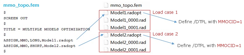
Рисунок 442:

Процесс оптимизации

PRADIOS анализирует все три колоды (оптимизация, стартовая и движковая колоды) для построения модели оптимизации. Для каждой итерации оптимизации будут записаны обновленный/оптимизированный файл стартера (<name>_rad_s#_i###_0000.rad) и файл движка (<name>_s#_i###_0001.rad), где ### — номер итерации оптимизации.

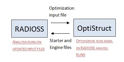
Рисунок 443: Обзор процесса оптимизации в PRADIOS

Обновленные файлы PRADIOS Starter и Engine будут решены PRADIOS, а результаты будут переданы в OptiStruct для обновления модели оптимизации OptiStruct.

Примечание: Для оптимизации топологии твердого тела с использованием PRADIOS оптимизация используется прямое управление плотностью. После завершения оптимизации топологии линейного статического отклика элементы твердого тела, имеющие значения от 0 до 1 в качестве переменных проектирования топологии, обновляются в конечно-элементной модели. Каждому твердотельному элементу конструкции напрямую назначается процент заполнения, значение которого равно связанной переменной топологии конструкции. Это использует опцию PRADIOS, /INIBRI/FILL, для сопоставления процента заполнения с переменной топологии конструкции.

Последовательность реализации

Следующие шаги иллюстрируют последовательный процесс, используемый для реализации оптимизации в PRADIOS:

1. Передайте файл оптимизации <name>.radopt в OptiStruct, используя синтаксис, указанный в Процессе оптимизации. OptiStruct автоматически выполнит поиск <name>_0000.rad и <name>_0001.rad в том же каталоге.

2. OptiStruct анализирует входные файлы PRADIOS, создает эквивалентную модель OptiStruct и продолжает выполнение этой модели OptiStruct.

3. OptiStruct применяет оптимизированные проектные переменные и записывает обновленные/оптимизированные файлы PRADIOS Starter/Engine (<name>_rad_s#_i###_0000.rad и <name>_s#_i###_0001.rad). В первом внешнем цикле проектные переменные еще не обновлены, а файлы Starter/Engine будут идентичны первоначальному вводу пользователя.

4. PRADIOS решает обновленные файлы Starter/Engine, сгенерированные на шаге 3.

5. OptiStruct считывает результаты PRADIOS, полученные на шаге 4, и запускает следующий запуск оптимизации (внутренний цикл).

6. Если результаты PRADIOS выходят за пределы порогового значения по сравнению с предыдущим внешним циклом, то процесс оптимизации не сошёлся.

7. Затем процесс оптимизации продолжается (с использованием метода ESLM) на обновленных результатах анализа PRADIOS, и генерируются новые оптимизированные проектные переменные. Шаги 3–6 повторяются для проверки сходимости процесса после последующей итерации. Если сходимость достигнута, переходите к шагу 8.

8. Процесс завершается, и выводятся оптимизированные результаты.

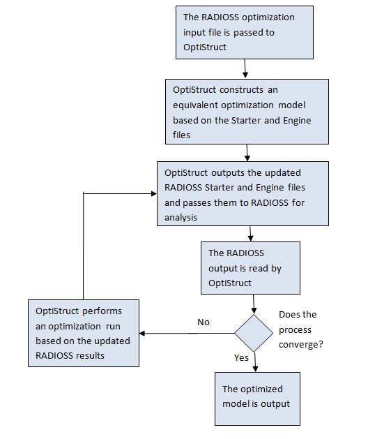
Рисунок 444: Последовательность оптимизации в PRADIOS и OptiStruct

База данных сообщений об ошибках

Этот раздел состоит из сообщений об ошибках в порядке возрастания номеров.

#1 по #299

Ошибка 119

ИДЕНТИФИКАТОР ОШИБКИ: 119
** ОШИБКА В ОПРЕДЕЛЕНИИ ИНТЕРФЕЙСА
ОПИСАНИЕ:
   -- ИДЕНТИФИКАТОР ИНТЕРФЕЙСА: 3
   -- НАЗВАНИЕ ИНТЕРФЕЙСА: контакт
   ЛАГРАНЖЕВА ПОВЕРХНОСТЬ ПУСТАЯ

Описание:

В 2D-анализе (\(N_{2D3D}\) =1 или 2 в /ANALY) вся сетка должна находиться в плоскости YZ и должна находиться в положительной оси Y и положительной оси Z. Если сетка находится в отрицательной оси Y или отрицательной оси Z, поверхность для контакта не найдена, и будет выведено это сообщение об ошибке.

Предложения по решению:

В препроцессоре (HyperMesh или HyperWorks) переместите всю сетку в положительную ось Y и положительную ось Z.

Ошибка 189

ИДЕНТИФИКАТОР СООБЩЕНИЯ: 189
** ОШИБКА: BEGIN НЕ ЯВЛЯЕТСЯ ДОПУСТИМЫМ КЛЮЧЕВЫМ СЛОВОМ
ИДЕНТИФИКАТОР СООБЩЕНИЯ: 189
** ОШИБКА: MAT НЕ ЯВЛЯЕТСЯ ДОПУСТИМЫМ КЛЮЧЕВЫМ СЛОВОМ

Описание:

Это сообщение обычно появляется, когда используется формат ввода одного файла, и не определены ключевые слова Engine.

Заголовок указывает “#PRADIOS STARTER”, используемый для файла Starter, и “# PRADIOS”, используемый для ввода одного файла (Starter и Engine в одном файле). Для ввода одного файла также необходимо завершить часть Engine с помощью “/END/ENGINE”.

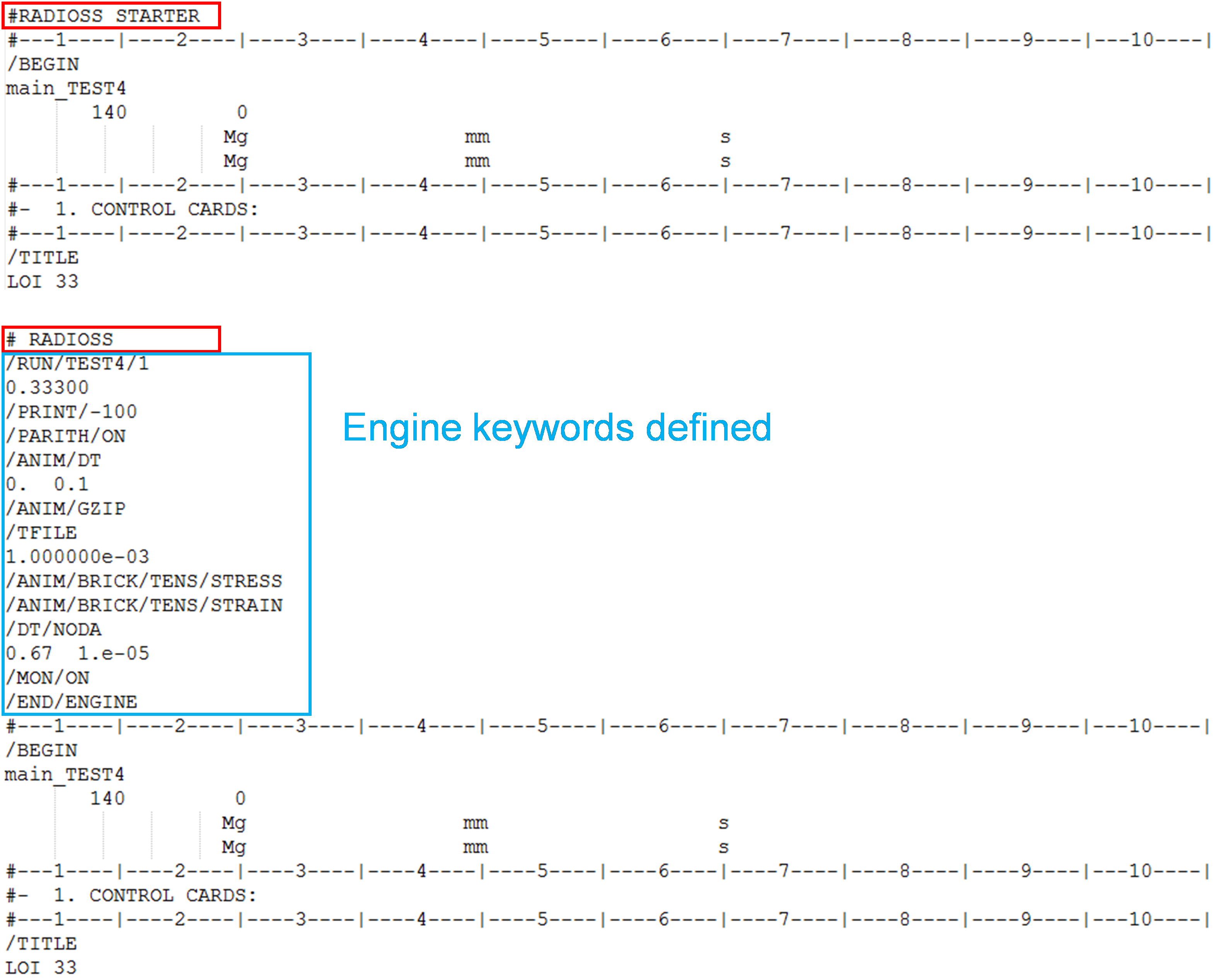
Рисунок 445:

Если заголовок указывает “# PRADIOS”, но Engine не определен, то возникает сообщение об ошибке с идентификатором 189.

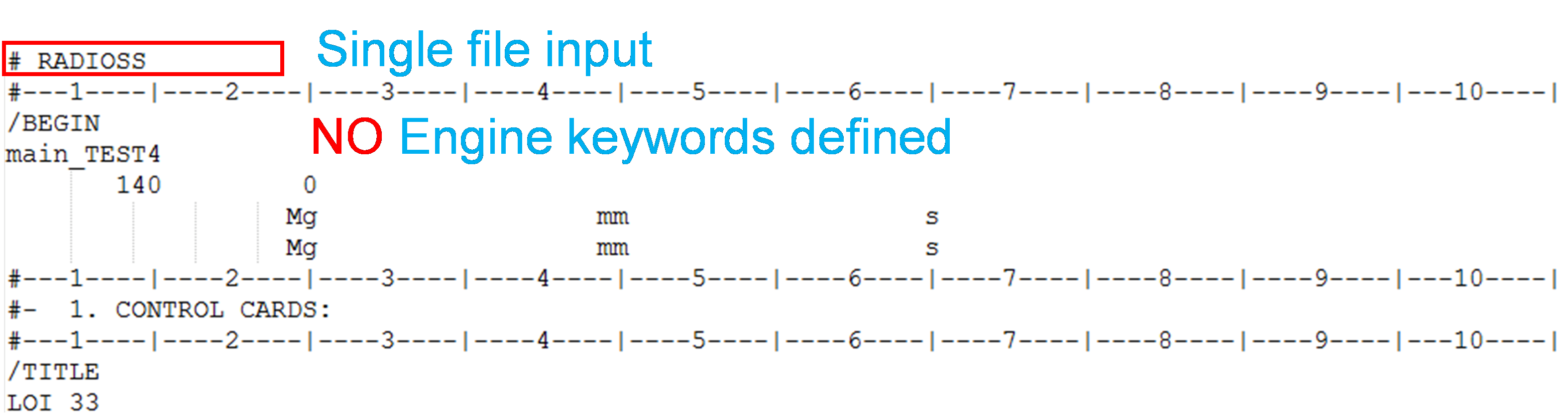
Рисунок 446:

Предложение по решению:

Используйте заголовок “#PRADIOS STARTER” или добавьте ключевые слова Engine.

Ошибка 197

ИДЕНТИФИКАТОР ОШИБКИ: 197
** ОШИБКА ВО ВХОДНЫХ ДАННЫХ
ОПИСАНИЕ :
-- ИДЕНТИФИКАТОР СВОЙСТВА : 521003304
  -- НАЗВАНИЕ СОБСТВЕННОСТИ: Новое ОБЪЕКТ 521003304
  НАПРАВЛЕНИЕ ОТСЧЕТА ПОЧТИ НОРМАЛЬНО ДЛЯ ОБОЛОЧКИ  ID=662193988

Описание:

Starter выведет это сообщение, когда направление, определенное в свойстве (опорный вектор / наклон), почти нормально к элементу оболочки.

Решатель предоставляет идентификатор свойства (в этом примере 521003304) и идентификатор элемента оболочки (в этом примере 662193988), для которого опорное направление почти нормально к элементу оболочки.

Решатель проецирует вектор V (или направление X наклона на элемент оболочки) вдоль нормали элемента оболочки (ниже левого рисунка). Если вектор V нормален к элементу оболочки, то проекция вектора на элемент оболочки не выполняется (проекция вектора V на оболочку составляет одну точку), и решатель не может определить направление 1 ортотропии (ниже правого рисунка), и появляется это сообщение об ошибке.

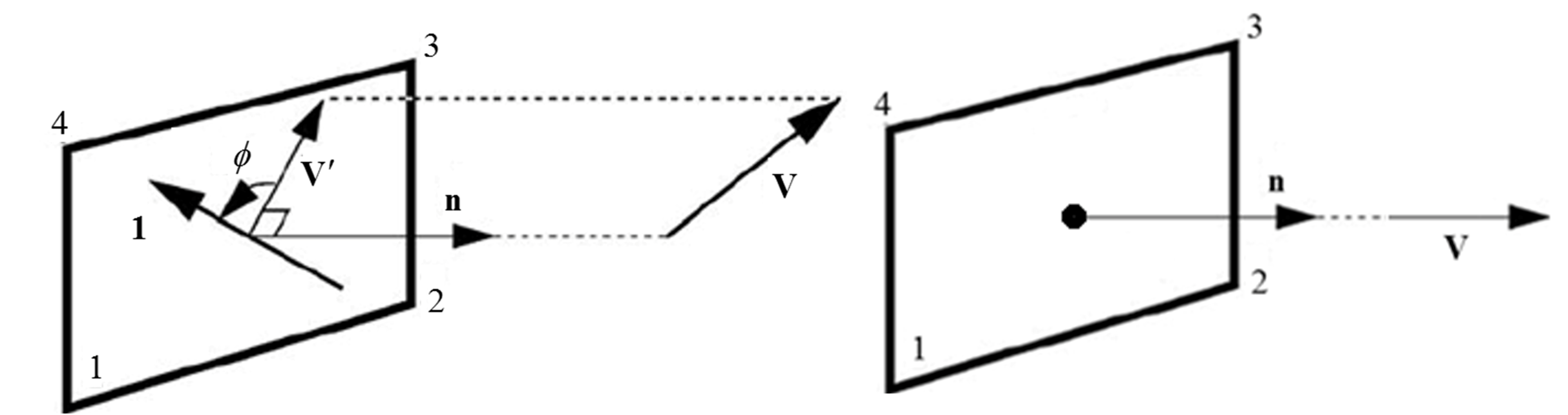
Рисунок 447:

Предложение по решению:

Направление вектора в свойстве, сообщенном Starter, необходимо изменить.

Примечание: Изменение направления вектора изменяет направление ортотропии.

Если материал на самом деле не ортотропный (E11=E22 и G12=G23=G31=E11/(2*(1+nu12)), изменение вектора не изменит результаты, и можно задать произвольный вектор (VX=VY=VZ=1).

Если материал ортотропный, вам нужно определить, что является направлением ортотропии, и ввести это направление в свойство. Если деталь имеет сложную геометрию, вам может потребоваться разделить деталь на разные секции и ввести вектор деки.

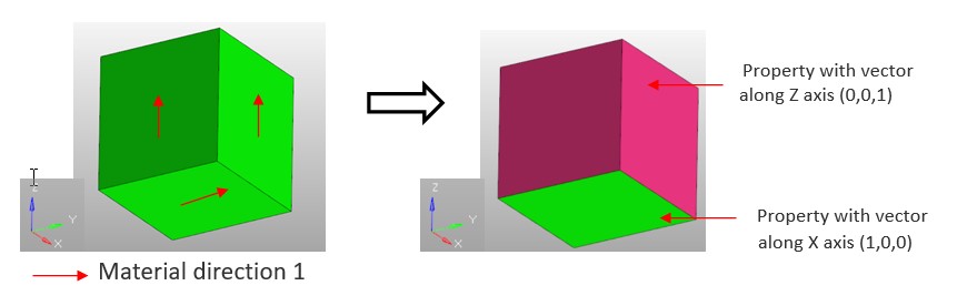
Рисунок 448:

Ошибка 223

ОШИБКА ID: 223
** ОШИБКА В ОПРЕДЕЛЕНИИ ЛУЧА

ОПИСАНИЕ :
  В ЛУЧЕ ID=1, N1 и N3 ИМЕЮТ ОДНО И ТО ЖЕ МЕСТОПОЛОЖЕНИЕ

РЕШЕНИЕ:
  ИЗМЕНИТЬ КООРДИНАТЫ N1 ИЛИ N3

ОПИСАНИЕ:

Элементам балки нужен узел ориентации (N3) для определения начального положения локальной рамки. Координаты этого узла (N3) должны отличаться от N1 и N2. Он также не может находиться на оси, определяемой N1N2.

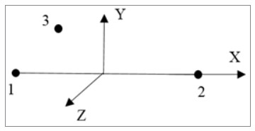
Рисунок 449:

Предложение по решению:

Эту проблему можно исправить вручную:

• Если поперечное сечение балки круглое или квадратное (Iyy=Izz), то всем элементам балки

можно назначить один и тот же N3. Главное требование — выбрать узел, который действителен для всех выбранных балок: N3 не должен лежать на оси ни одной из выбранных балок.

• Если Iyy≠Izz, то же самое, узел N3 все еще можно назначить нескольким элементам балки,

если их локальная ось X похожа (определяется N1-N2). Если локальная ось X балки не похожа, то выберите разные N3 для разных балок: N3 не должен лежать на оси балки.

#300 по #699

Ошибка 480

ИДЕНТИФИКАТОР ОШИБКИ: 480
** ОШИБКА В МАТЕРИАЛЬНОМ ЗАКОНЕ
ОПИСАНИЕ :
- ИДЕНТИФИКАТОР МАТЕРИАЛА: 521002880
- НАЗВАНИЕ МАТЕРИАЛА: По умолчанию MAT24 MAT_PIECEWISE_LINEAR_PLASTICITY.2
EPS_T ДОЛЖЕН БЫТЬ СТРОГО МЕНЬШЕ EPS_M

Описание:

В материалах LAW27 и LAW36 при определении отказа при растяжении существуют определенные правила, которым следует следовать. В этом примере решатель сообщает, что для материала 521002880 это недопустимо.

Предложение по решению:

Пример LAW36: Eps_t < Eps_m < Eps_f

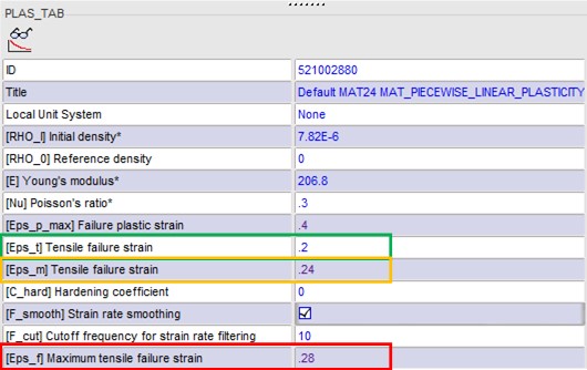
Figure 450:

LAW27 Пример:

EPS_t1 < EPS_m1 < EPS_f1

EPS_t2 < EPS_m2 < EPS_f2

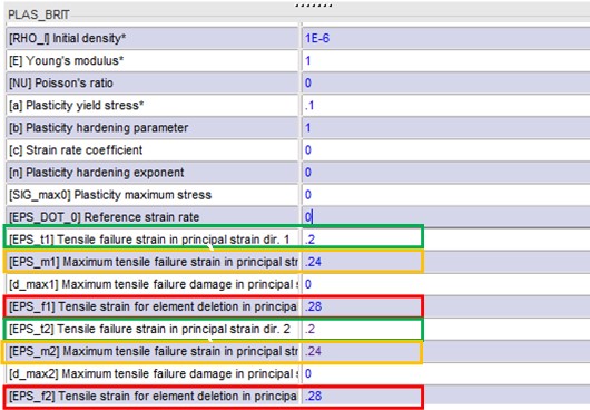
Рисунок 451:

Ошибка 592

ОШИБКА ID :           592
** ОШИБКА в формате входной колоды N STARTER
ОПИСАНИЕ:
ВХОДНАЯ ВЕРСИЯ=0
СТРОКА: /VERS/2017 РЕШЕНИЕ:
/BEGIN КАРТА ОБЯЗАТЕЛЬНА ДЛЯ STARTER ВХОДНАЯ ВЕРСИЯ >= 50

Описание:

Решатель ожидает карту /BEGIN, но вместо этого нашел другое ключевое слово. Пример: /VERS/2017

Наиболее распространенные причины появления этого сообщения:

• Заголовок указывает на отдельные файлы Starter и Engine, но файл Engine присутствует под заголовком.

• Отсутствует /BEGIN или /END.

Ошибка 611

ИДЕНТИФИКАТОР СООБЩЕНИЯ: 611

** ОШИБКА В НАЧАЛЬНОМ ПРОНИКНОВЕНИИ В ИНТЕРФЕЙСЕ ОПИСАНИЕ: 189 - ИДЕНТИФИКАТОР ИНТЕРФЕЙСА: 11 - НАЗВАНИЕ ИНТЕРФЕЙСА: Глобальный интерфейс Зазор 0,49 Только оболочки INACTI = 6 НЕВОЗМОЖНО ИЗМЕНИТЬ КООРДИНАТЫ УЗЛА ВТОРИЧНОГО УЗЛА: 823868424 ** НАЧАЛЬНОЕ ПРОНИКНОВЕНИЕ = 0,4900000e+00 НЕВОЗМОЖНО ВЫЧИСЛИТЬ НОВЫЕ КООРДИНАТЫ ВТОРИЧНОГО УЗЛА******

Описание:

Решатель выведет это сообщение, когда не сможет вычислить новые возможные координаты узла, который изначально проникает. Решатель предоставит следующую информацию:

• Идентификатор узла, для которого не удалось вычислить новую позицию (в этом примере: 823868424)

• Идентификатор интерфейса (в этом примере: 11)

Предложения по решению:

В HyperCrash или HyperMesh проверьте начальное проникновение для идентификатора интерфейса, для которого возникла ошибка. Отсортируйте начальное проникновение по минимальному остаточному расстоянию (столбец Res. Dist.).

В большинстве случаев узлы, для которых Starter не сможет вычислить новую позицию, будут узлами, где остаточное расстояние равно 0. Это означает, что узлы изначально находятся на основном сегменте.

Выберите эти узлы в списке и выделите их на дисплее ( в HyperMesh).

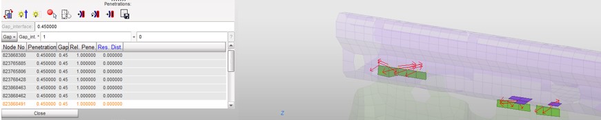
Рисунок 452:

Существуют три распространенные ошибки моделирования, которые могут привести к этому типу проблем.

1. Пружины, представляющие сварные швы или болты, включены в глобальный контакт. Их следует удалить.

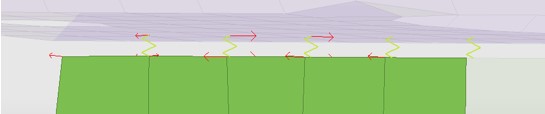
Рисунок 453:

2. Проблема сетки:

В области, где в сетке есть трещины, узлы должны быть эквивалентны (с помощью HyperMesh).

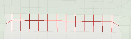
Рисунок 454:

Поверх твердой сетки находится кожа, а узлы кожи/твердого тела не эквивалентны. Узлы должны быть эквивалентны (с HyperMesh).

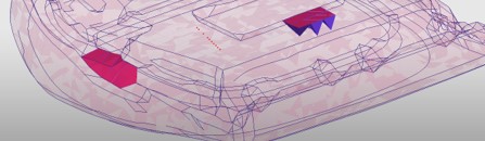
Рисунок 455:

3. Твердый контакт с твердым с нулевым зазором. Это не поддерживается интерфейсом TYPE7, TYPE11 или TYPE19. Либо переместите узлы, чтобы создать зазор (0,1 мм), либо используйте интерфейс TYPE24. ..

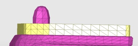
Рисунок 456:

#700 через #1199

Ошибка 953

ИДЕНТИФИКАТОР ОШИБКИ: 953
** ОШИБКА ПРИ ЧТЕНИИ ПАРАМЕТРОВ
ОПИСАНИЕ:
НЕОЖИДАННЫЙ КОНЕЦ ФАЙЛА

ИДЕНТИФИКАТОР ОШИБКИ: 968
** ОПИСАНИЕ ОШИБКИ ВВОДА:
ОШИБКА ПРИ ЧТЕНИИ ВХОДНОГО ФАЙЛА STARTER

Описание:

Эта ошибка обычно возникает, когда параметры присутствуют во входных данных, а в конце файла отсутствует /END.

В большинстве случаев это происходит, когда задание было отправлено до завершения копирования в рабочий каталог.

Предложения по решению:

Добавьте /END в конец входного файла или завершите копирование всех входных файлов.

Ошибка 958

ИДЕНТИФИКАТОР ОШИБКИ: 958
** ОШИБКА ВО ВРЕМЯ ОЦЕНКИ ПАРАМЕТРОВ
ИДЕНТИФИКАТОР ОШИБКИ: 952
** ОШИБКА В ФОРМАТЕ ВХОДНОЙ КОЛОДЫ СТАРТЕРА
ОПИСАНИЕ:
ВЕРСИЯ ВХОДА=0
LINE : /PARAMETER/GLOBAL/INTEGER/6620015

Описание:

Эта ошибка возникает, когда решатель не может оценить значение параметра. Обычно это происходит, когда выражение не завершено (проверьте значение выражения в HyperCrash) или в выражении есть некоторые параметры, на которые есть ссылки, и они не определены в модели.

Предложение по решению:

Параметр “Time1” равен “ActTTF” + 20. Параметр “ActTTF” не определен, поэтому решатель не может оценить значение “Time1”.

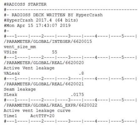
Рисунок 457: Пример

Ошибка 1078

ИДЕНТИФИКАТОР ОШИБКИ: 1078
\*\* ОШИБКА: СВЯЗАННЫЙ ИНТЕРФЕЙС
ОПИСАНИЕ :
 -- ИДЕНТИФИКАТОР ИНТЕРФЕЙСА: 1
 - НАЗВАНИЕ ИНТЕРФЕЙСА: новый контакт
 1 ВТОРИЧНЫЙ УЗЕЛ(Ы) ДЕАКТИВИРОВАНЫ ИЗ ИНТЕРФЕЙСА
 ВТОРИЧНЫЙ УЗЕЛ: 82 НЕ НАЙДЕНО ГЛАВНОГО СЕГМЕНТА В ДИАПАЗОНЕ 1.0000000000000E-02

Описание:

Решатель выведет это сообщение, когда узел включен в интерфейс TYPE2 и не найден основной сегмент в пределах расстояния поиска для этого узла, а флаг «Игнорировать» установлен на 1000.

Решатель предоставит идентификатор интерфейса (в этом примере 1) и идентификатор узла (в этом примере 82), для которого решатель не нашел основной сегмент в пределах расстояния поиска (1.0e-2 в этом примере).

Проверка модели HyperCrash обнаруживает этот тип ошибки (вторичные узлы без проекта).

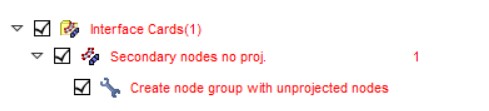
Рисунок 458:

Предложения по решению:

Есть несколько способов решения этой проблемы:

• Используйте Ignore = 1, если эти узлы не нужно привязывать, или удалите эти узлы из интерфейса TYPE2.

• Переместите узлы, которые не находят проекцию, так, чтобы они попадали в расстояние поиска.

• Немного увеличьте расстояние поиска (\(D_{search}\)).

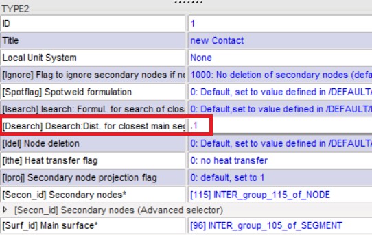
width

4.51706in

height

2.85858in

Рисунок 459:

Ошибка 1104

ИДЕНТИФИКАТОР ОШИБКИ: 1104
** ОШИБКА ПРИ ПОСТРОЕНИИ ПОВЕРХНОСТИ ИЗ ДЕТАЛЕЙ ТВЕРДОГО ТЕЛА
ОПИСАНИЕ:
--ИДЕНТИФИКАТОР ПОВЕРХНОСТИ: 830005865
--НАЗВАНИЕ ПОВЕРХНОСТИ: Новый SURF 830005865
НЕДОСТУПНЫЙ ПАРАМЕТР /SURF/PART/Surf_ID ДЛЯ СОЗДАНИЯ ПОВЕРХНОСТИ
РЕШЕНИЕ:
ДЛЯ ЧАСТИ ТВЕРДОГО ТЕЛА
ИСПОЛЬЗУЙТЕ /SURF/PART/EXT/Surf_ID или /SURF/PART/ALL/Surf_ID

Описание:

Решатель выведет это сообщение, когда PART с твердыми элементами включен в /SURF/PART. Это ключевое слово позволяет строить поверхности только из 2D-элементов, а не 3D.

Предложения по решению:

1. Запустите проверку с именем Volumic Parts in Surf в HyperCrash Model Checker.

2. Выберите Switch to Surf Ext или Switch to Surf All, чтобы автоматически переключить ключевое слово на /SURF/PART/EXT или /SURF/PART/ALL. ..

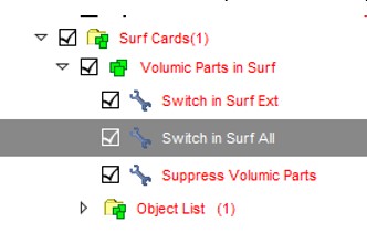
Рисунок 460:

Ошибка 1130

 ИДЕНТИФИКАТОР ОШИБКИ: 1130
 ** ОШИБКА В ИНТЕРФЕЙСЕ ПОЛЬЗОВАТЕЛЯ
 ОПИСАНИЕ:
 ОПЦИЯ: /MAT/USER1
 ИСПОЛЬЗОВАНА ОПЦИЯ ИНТЕРФЕЙСА ПОЛЬЗОВАТЕЛЯ, НО ПРОЦЕДУРА ИНТЕРФЕЙСА ПОЛЬЗОВАТЕЛЯ НЕ НАЙДЕНА

Описание:

Стартер выведет это сообщение, когда он прочитает пользовательский материал (LAW29), а пользовательская библиотека, определяющая поведение и формат этого материала, не определена.

Предложения по решению:

Замените пользовательский материал любым другим совместимым и поддерживаемым ключевым словом PRADIOS material.

ОШИБКА МАССЫ ИЛИ ЭНЕРГИИ ИЗ-ЗА КОНТАКТА

::

**ПРЕДУПРЕЖДЕНИЕ МИНИМАЛЬНЫЙ ШАГ ВРЕМЕНИ 0.248E-04 В ИНТЕРФЕЙСЕ 11(DTMIN= 0.2500E-04) УДАЛЕН ВТОРИЧНЫЙ УЗЕЛ 63086879 ИЗ ИНТЕРФЕЙСА

ИДЕНТИФИКАТОР СООБЩЕНИЯ: 206 ** ЗАПУСК ОСТАНОВЛЕН: ДОСТИГНУТ ПРЕДЕЛ ОШИБКИ ЭНЕРГИИ

*** УЗЕЛ С НАИБОЛЬШИМ ИЗМЕНЕНИЕМ МАССЫ

Описание:

В нескольких случаях моделирование может завершиться ошибкой ERROR, поскольку слишком много массы добавлено для поддержания постоянного временного шага контакта.

Почему необходимо добавлять массу для поддержания стабильности контакта?

• Временной шаг постоянен, когда используются /DT/NODA/CST, /DT/NODA/CST2 или /DT/INTER/CST.

• Временной шаг интерфейса вычисляется как \(\Delta t\frac{2m}{K}\)

Жесткость увеличивается в зависимости от проникновения \(K=K_{0}\frac{Gap^{2}}{(Gap-p)^{2}}\)

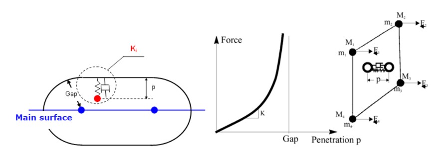
Рисунок 461:

По мере увеличения проникновения в контакте увеличение жесткости приводит к увеличению массы для поддержания постоянного временного шага.

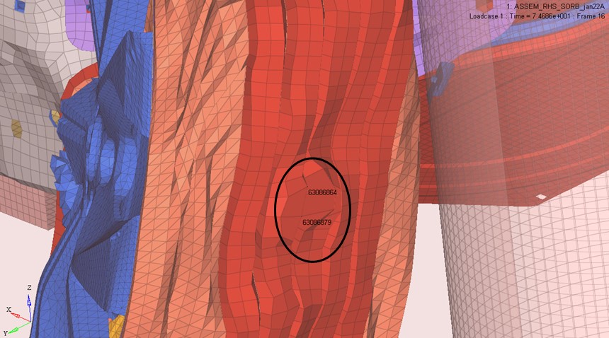
Рисунок 462:

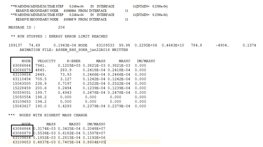
Рисунок 463:

Например, шина упирается в жесткий барьер. За шиной тормозной диск (или калибр) прижимает шину к барьеру. Глобальный контакт недостаточно жесткий и приводит к большим проникновениям.

◦ Жесткость увеличилась

◦ Масса добавляется для поддержания постоянного шага времени

Предложения по решению:

Типичным решением этой проблемы является создание локального контакта с большим зазором и жесткостью. Увеличение начальной жесткости приводит к меньшему временному шагу в начале проникновения, но это увеличит временной шаг, если проникновение большое.

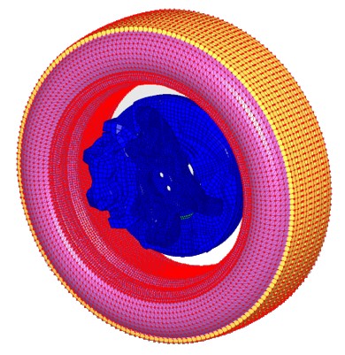
Рисунок 464: Локальный контакт

Контакт между двумя жесткими частями возможен с интерфейсом TYPE7 и TYPE11 или TYPE19. Основная проблема заключается в том, что он создаст глубокие проникновения в контакт, что может привести к добавлению массы для поддержания временного шага на значении, указанном в /DT/NODA/CST или /DT/NODA/CST2.

Есть два решения для решения этого типа проблемы:

• Переключить хотя бы одну из частей на деформируемую

• Добавить локальный контакт с большим зазором и жесткостью

ОШИБКА МАССЫ ИЛИ ЭНЕРГИИ ИЗ-ЗА ВЫСОКОГО ИСКАЖЕНИЯ

*** УЗЛЫ С НАИБОЛЬШЕЙ СКОРОСТЬЮ

*** УЗЛЫ С НАИБОЛЬШИМ ИЗМЕНЕНИЕМ МАССЫ

Описание:

При очень большой пластической деформации моделирование может стать нестабильным и завершиться с ошибкой ERROR из-за ошибки энергии или массы.

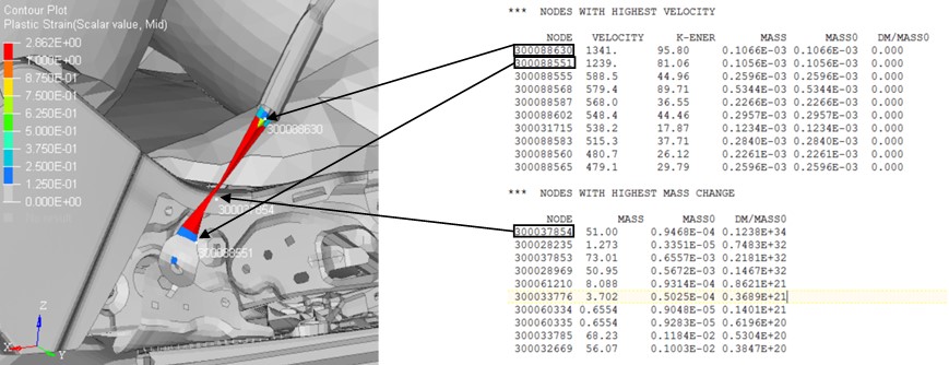
Рисунок 465:

Предложение по решению:

На основе результатов существуют различные способы решения этой проблемы:

• Определите правильное разрушение деформации

• Материал может быть неправильным (система единиц) или типом (пластик вместо стали, предел текучести слишком низкий…)

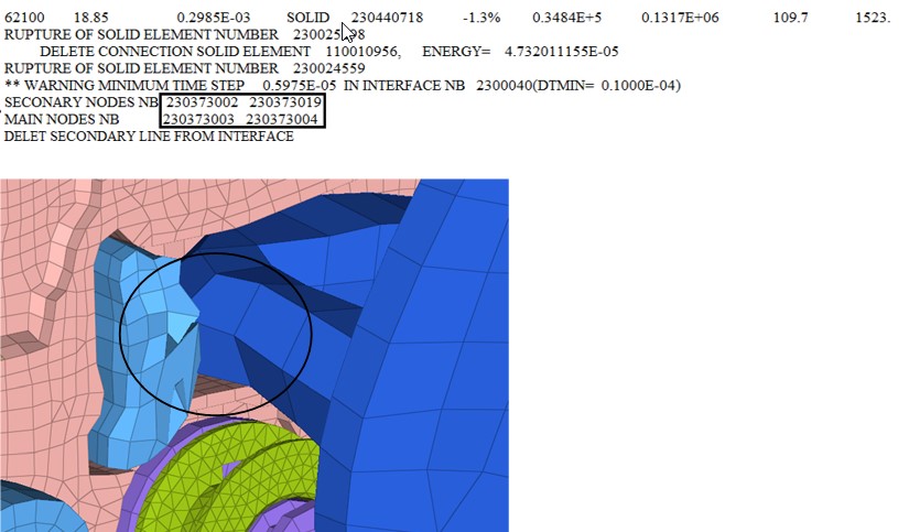
Рисунок 466:

Изначально есть пересечение, которое создает локальное искажение. Чтобы решить эту проблему, исправьте пересечение и определите правильное разрушение деформации в материале.

ПРЕДУПРЕЖДЕНИЕ ID :          542
** ПРЕДУПРЕЖДЕНИЕ. ИНЕРЦИЯ ЖЕСТКОГО ТЕЛА
ОПИСАНИЕ :
- ИДЕНТИФИКАТОР ЖЕСТКОГО ТЕЛА : 713264
- НАЗВАНИЕ ЖЕСТКОГО ТЕЛА : NULL
НЕФИЗИЧЕСКАЯ ИНЕРЦИЯ:
ГЛАВНАЯ ИНЕРЦИЯ 150,0050404753 СОЗДАЕТ СУММУ
ДВУХ ДРУГИХ 0.60340391378794E-02 + 0.3645995262784E-02

Описание:

Когда инерция твердого тела не является физической, твердое тело может стать неустойчивым. Когда инерция твердого тела не является физической, PRADIOS выведет предупреждение в Starter.

Если эти предупреждения не будут исправлены, может произойти следующее:

• Жесткое тело становится нестабильным и движется с очень высокой скоростью в транспортном средстве

• Жесткие вторичные узлы все еще находятся в глобальном контакте и будут генерировать нереалистичную деформацию

• Численные проблемы, так как скорость удара очень высокая (>1500 м/с)

Предложение по решению:

Исправьте нефизическую инерцию твердого тела.

ОТРИЦАТЕЛЬНАЯ ИНЕРЦИЯ ИЛИ ЖЕСТКОСТЬ

NEGATIBE INERTIA НА УЗЛЕ ID=823767293

Описание:

Эта проблема обычно чаще возникает в PRADIOS v12.x, чем в более поздних версиях (2017.x). Она возникает, когда узел интерфейса TYPE2 выступает за пределы ближайшего основного сегмента. Ошибка связана не с высотой вторичного узла относительно основного сегмента, а с тем, что его проекция находится за пределами основного сегмента.

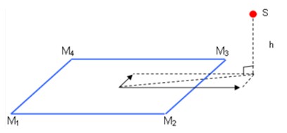
Рисунок 467:

Предупреждение в Starter печатается для узлов, которые выступают за пределы основного сегмента.

ИДЕНТИФИКАТОР ПРЕДУПРЕЖДЕНИЯ: 345
** ПРЕДУПРЕЖДЕНИЕ: ПРОВЕРЬТЕ СВЯЗАННЫЙ ИНТЕРФЕЙС
ОПИСАНИЕ:
-- ИДЕНТИФИКАТОР ИНТЕРФЕЙСА: 557392358
--- НАЗВАНИЕ ИНТЕРФЕЙСА: CONNECTION.37
8238684 2 823767497 823767293 823767296 823767504 -1.279664112565 -0.9934883789504 0.7066172931858

Используйте HyperCrash Model Checker для проверки «Вторичные узлы без выступающих». Это позволяет идентифицировать узлы, которые выступают за пределы ближайшего основного сегмента.

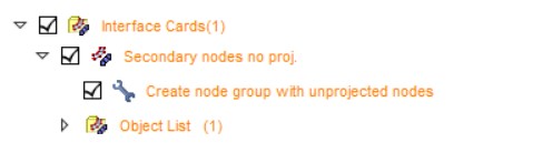
Рисунок 468:

Предложение по решению:

Есть несколько способов решения этой проблемы:

• Удалите узлы, которые выступают за пределы ближайшего основного сегмента из интерфейса TYPE2

• Переместите узлы так, чтобы они больше не выступали за пределы сегмента

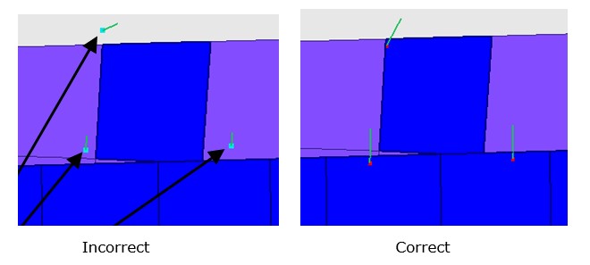
Рисунок 469:

Этот раздел состоит из предупреждающих сообщений в порядке возрастания номеров.

#100 по #699

ПРЕДУПРЕЖДЕНИЕ 194

ПРЕДУПРЕЖДЕНИЕ ID :           194
** ПРЕДУПРЕЖДЕНИЕ В ИЕРАРХИИ ССЫЛКА
ОПИСАНИЕ :
-- ПОВЕРХНОСТЬ ID : 8300005857
-- INTER_group_830006186_of_PART_TITLE : ЧАСТЬ
ССЫЛКА НА НЕСУЩЕСТВУЮЩИЙ ИДЕНТИФИКАТОР=600000000

Описание:

Starter выведет это сообщение, когда объект (узел, элемент, часть, подмножество) определен в группе узлов, элементов, поверхностей или линий, но не существует в модели.

В приведенном выше примере идентификатор детали 600000000 определен в поверхности 830005857. Эта часть не существует в модели. Объекты, на которые есть ссылки, но которые не определены в модели, будут показаны в HyperCrash в обозревателе моделей как «Неразрешенные идентификаторы».

Рисунок 470:

Предложения по решению:

Удалите группу или выберите объект для переопределения группыp.

ПРЕДУПРЕЖДЕНИЕ 542

| ПРЕДУПРЕЖДЕНИЕ ID : 542
| ** ПРЕДУПРЕЖДЕНИЕ ИНЕРЦИЯ ЖЕСТКОГО ТЕЛА

ОПИСАНИЕ : | – ЖЁСТКОЕ ТЕЛО ID : 136849917 | – НАЗВАНИЕ ЖЕСТКОГО ТЕЛА: MAT_RIGID_1500016_PART_325 НЕФИЗИЧЕСКАЯ ИНЕРЦИЯ: | ГЛАВНАЯ ИНЕРЦИЯ 249,2162969709 БОЛЬШЕ, ЧЕМ СУММА | ИЗ ДВУХ ДРУГИХ 112.70695453317 + 48.42692228428

Описание:

Стартер выведет это сообщение, когда инерция не является физической. В большинстве случаев это происходит, когда:

1. Инерция была определена, но неправильно в случае Icog=3 и 4.

2. Постоянная инерция была определена (50) для Jxx, Jyy, Jzz, Jxy, Jxz и Jyz, а Isphere не установлен на 1.

Это предупреждение необходимо исправить, так как оно может вызвать проблемы во время Двигателя. Это можно исправить в HyperCrash.

Предложение по решению:

Для случая 2 выше простой способ решения — использовать HyperCrash. Столбец инерции отображается на панели жестких тел, выберите все жесткие тела с Jxx, Jyy, Jzz = 50 и установите Jxy, Jyz, Jxz = 0.

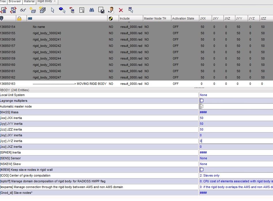
Рисунок 471:

#700 по #1199

Ошибка 1079

ИДЕНТИФИКАТОР ПРЕДУПРЕЖДЕНИЯ: 1079

** ПРЕДУПРЕЖДЕНИЕ: ПРОВЕРЬТЕ СВЯЗАННЫЙ ИНТЕРФЕЙС ОПИСАНИЕ:

– НАЗВАНИЕ ID: 1 – НАЗВАНИЕ ИНТЕРФЕЙСА: новый Контакт ОТНОСИТЕЛЬНО 1 УЗЛА(S)

ВТОРИЧНЫЙ УЗЕЛ: 82 БЛИЖАЙШИЙ СЕГМЕНТ: 1 ГЛАВНЫЙ УЗЕЛ: 146 145

142 143

S = 1.400000000000 T = 1.160000000000 DIST = 2.9393876913398E-02

Описание:

Это сообщение означает, что проекция вторичного узла с идентификатором 82 находится вне основного сегмента, но PRADIOS рассматривает проекцию как перемещение этого вторичного узла на ближайший край сегмента. S и T являются расстоянием локального направления ‘s’ и ‘t’.

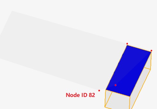
Рисунок 472:

Индекс

Специальные символы

-check аргумент (начальный) 21

-dylib [FILE] аргумент (начальный) 22, 27

-help аргумент

Двигатель 23

Стартер 19

-аргумент HSTP_READ (Стартер) 22

-аргумент HSTP_WRITE (Стартер) 22

-аргумент mds libpath [PATH] (Стартер) 22, 27

-аргумент norst (Движок) 26 -notrap argument

Двигатель 26

Стартер 20

-nspmd [номер домена spmd] аргумент (Стартер) 20

-outfile аргумент

Двигатель 26

Стартер 21

-rseed (seed] аргумент (Стартер) 22

-rxalea (xalea] аргумент (Стартер) 22

-version аргумент

Двигатель 24

Стартер 19

A

Файлы ABF 542 расширенное масштабирование массы .out примеры файлов 70 автомобильный пример 59 текущие возможности и ограничения 53 формовка металла пример 70 рекомендуемый контрольный список 56

расширенные методы 32 требования к модели подушки безопасности 389 моделирование подушки безопасности развертывание отладки 429 управление шагом времени элемента 388 FVMBAG1 руководящие принципы 389 контролируемый объем 379 рекомендация по настройке 426 бак тест 422

подушка безопасности, материал ткани 393 подушка безопасности, метод конечного объема 399 подушка безопасности, начальный воздух внутри 393

Формула ALE 491

580

Расчет сетки ALE 499

Интерфейсы ALE 508

Ключевые слова ALE, резюме 487 Материалы ALE/CFD 501 Файлы анимации 542 Приложение 453 Область применения 389 Произвольный Лагранжево-Эйлерово (ALE) 487 Искусственное демпфирование для ударных волн 507 Предупреждение о зазоре автоконтакта 368 Автоматическое создание поддомена 538

B

Плохой объем, исключить 421 Энергия баланса 445 Масса баланса 445 Импульс баланса 445 Основные соотношения 453 Моделирование болтов для столкновения 323 Натяжение болтов 374

C

контрольные единицы 442 файл контрольной точки 35 классические элементы балки (/PROP/BEAM) 93 аргумент командной строкиt

Двигатель 22

Starter 18 общие проблемы, интерфейс TYPE3 и TYPE5 350 связь между AcuSolve и PRADIOS 465, 479 связь между доменами - единый формат входного файла 538 связь между PRADIOS и AcuSolve 470 композитная модель отказа 294 материал 265 моделирование 279 свойства 280 composite material

LAW12 и LAW14 266

LAW19 и LAW58 277

LAW25 (Tsai-WU и CRASURV) 272 композитные свойства элементы оболочки 280 твердотельный элемент 292

вычислительная гидродинамика (CFD) 487 компьютерный кластер 29

материалы бетона

/MAT/LAW10 and /MAT/LAW21 212

/MAT/LAW24 216

/MAT/LAW81 232 соединение между доменами, формат файла с несколькими входами 546 контакт между доменами, формат файла с несколькими входами 548 контакт между Sol2SPH и другими частями 531 контактный интерфейс шаг по времени управление 49

контактный интерфейс, неявный структурный конечноэлементный анализ 459 контактная обработка метод множителей Лагранжа 345 контактная обработка метод штрафа 345 контрольный файл (C-файл) 32 система координат

система материалов 154

Выделение ЦП формат файла с несколькими входами 550 формат файла с одним входом 543

текущие возможности и ограничения 53 текущие ограничения, формат файла с одним входом 545 цилиндрическое соединение 336

D

dashpot - формулировка жесткости 116 ввод данных формат файла с несколькими входами 549 формат файла с одним входом 541

dc-fsi с использованием PRADIOS и AcuSolve 466 DC-FSI с использованием PRADIOS и AcuSolve 465, 479 рекомендации по отладке проверки вычислений 445 модель отладки 447 проверка модели 444 инструментарий модели 443 подготовка модели 433 согласованность единиц 438

оптимизация конструкции реализация 555 процесс 557 оптимизация запуска 556 установка переменных среды 556

различное количество ядер 30 соединение дифференциала 339 диффузный образование шейки, нестабильность материала 261 устойчивость условия Дрюкера проверить 187 модель пластичного разрушения

/FAIL/BIQUAD 239

/FAIL/JOHNSON 237

E

блокировка удара край-в-край 367 упругий пластик кусочно-линейный материал - /MAT/LAW36 206 упругопластические материалы 202 упругопластические материалы - Джонсон-Кук (/MAT/LAW2) 202 элемент обработка отказов 259 формулы элементов, неявный структурный конечно-элементный анализ 458 рекомендации по выбору элемента 91

управление шагом времени элемента 47

элементарные граничные условия 505 элементы твердые 82 элементы твердотельные оболочки 84 энергетический баланс 445

файл двигателя, неявные примеры анализа 485

входные данные двигателя

руководство пользователя 515 база данных сообщений об ошибках 560, 577 формулировка Эйлера 491 коды выхода (стартер и двигатель) 17 явный структурный конечно-элементный анализ 37

F

модели отказов для пластичных материалов 236 отказ, явный структурный анализ конечных элементов 236

-входной [файл] аргумент

Двигатель 24

Starter 19 фильтрация, приложение 455 конечные элементы 82 первые проверки во время/после вычисления 445 моделирование жидкости и жидкости-конструкции 487 анализ взаимодействия жидкости-конструкции с AcuSolve и PRADIOS 465, 479 соединение жидкости/конструкции 493 взаимодействие жидкости/конструкции, интерфейс ALE/Лагранжа 512 сила и момент - жесткость пружины 96 вычисление силы и момента, инструменты моделирования 164 трение 360

Подушка безопасности FVM, автономный запуск 418

Контрольный список подушки безопасности FVMBAG1 421 пористость ткани 406 корпус 411 внутренние контакты 409 запуск стабильности 416

G

генератор газа 391 общие рекомендации - временной шаг 79 генерация тангенциальной силы 367 глобальный временной шаг 39

H

теплообмен 364 Материалы HILL - Руководство пользователя 208 песочные часы формулы 147 гиперэластичные материалы

/MAT/LAW42 178

/MAT/LAW62 (VISC_HYP) 182

/MAT/LAW69 184

/MAT/LAW82 186

/MAT/LAW88 189

/MAT/LAW92 (Arruda-Boyce) 192

/MAT/LAW92 (Yeoh) 195*Бергстром-Бойс *196 заключение 191 Огден 177 I

реализация, оптимизация дизайна 555 неявный анализ активация 461 неявный конечно-элементный анализ приложение 485 неявный конечный выходные сообщения анализа элементов 481 неявный конечно-элементный анализ устранение неполадок 483 неявные решатели с параллельной версией, совместимость 463 неявный структурный конечно-элементный анализ 457 несовместимые кинематические условия 342 непоследовательная жесткость, пружины 117 увеличение скорости вычислений и поддержание точности 50 увеличение массы 365 начальные проникновения 355 интерфейс вытяжной валик (/INTER/TYPE8) 369 интерфейс край-к-краю (/INTER/TYPE11) 371 интерфейс общего назначения (/INTER/TYPE7) 353 интерфейс несимметричный (/INTER/TYPE5) 348 жесткость интерфейса 358

интерфейс симметричный (/INTER/TYPE3) 347 интерфейс управление шагом по времени 365 интерфейс TYPE6 (/INTER/TYPE6) 352 интерфейсы явный конечный элемент 344 интерфейсы, ALE 508

J

Матрица Якоби 144

K

метод штрафа кинематических условий 341 кинематические условия, неявные структурный конечноэлементный анализ 459 кинематические ограничения 326, 507

L

Формулировка Лагранжа 491 запуск многодоменного анализа многодоменный формат входного файла 550

запуск многодоменного анализа единый формат входного файла 543

LAW12 и LAW14, композитный материал 266 линейные решатели 463 нагрузки, неявные особенности и совместимость 459 локальная система плоскости сечения, инструменты моделирования 163 угол наклона, отказ 251

M

баланс масс 445 совместимость материалов, неявная структура конечно-элементный анализ 458 неустойчивость материала, диффузное сужение 261 материалы, явная структурная КЭА 172 рекомендации по сетке 144 сетка и складывание 389 методология

Очистка САПР 494 методы применения кинематических условий 341 модель настройка многодоменный 535 формат множественного входного файла 546 формат единого входного файла 537

размер модели, несколько ядер 30 руководства по моделированию, Sol2SPH 531 инструменты моделирования, перекос и рамка 159 баланс импульса 445

контролируемый объем

AIRBAG1 тип 380

COMMU1 тип 384

FVMBAG1 тип 387

GAS тип 387

LFLUID тип 388 PRES тип 388 шаг времени 388

самые популярные единицы 442 mpi и параметры PRADIOS когерентность 26 многодоменный

настройка модели 535

многодоменная техника 533 многоточечные ограничения (/MPC) 339 несколько ядер 29 несколько файлов движка 34 формат файла множественного ввода, PRADIOS 546

N

новые элементы балки (/PROP/INT_BEAM) 93 узловые граничные условия 504 узловой временной шаг 38 управление узловым временным шагом 44 нелинейный анализ с контактом 476 нелинейные неявные примечания к анализу 476 нелинейные решатели 464

аргумент nspmd [номер домена spmd] (стартер) 20

O

другие руководства по моделированию, Sol2SPH 531 выходные данные, формат одного входного файла 542

P

предварительная загрузка

натяжение болта 374 определить 375

пружина шкива TYPE12 129

Q

квадратичный контакт поверхности 372 квазисжимаемая опция 503 квазистатические примечания к анализу 475 квазистатическое моделирование - временной шаг 81

R

реечное соединение 339 пример входного файла RAD2RAD 553

выходной файл RAD2RAD 542 распараллеливание RAD2RAD 552 опорная геометрия 390 жесткое тело, /RBODY 326 жесткое звено, /RLINK 338 жесткая стена, /RWALL 330 вращательное соединение типа шестерни 339 запуск исполняемых файлов напрямую 16 параметры запуска

Скрипт моделирования Laduga 16

Вычислительная консоль 11

HyperMesh 16 run PRADIOS 11 rupture interface 369

S

scaling failure strain 256 section cutting plane, modeling tools 161 section output, modeling tools 170 sections (/SECT) 160 select main and secondary sides, fluid/fluid interface 510 shell elements

/PROP/SHELL 86

формат файла с одним входом 537 вычисление с одинарной точностью 35 перекос и рамка 159 распределение ячеек сглаженной гидродинамики частиц (SPH) 518 максимальное сохраненное число соседей 522 условия симметрии 523

-nthread [номер потока smp] аргумент

Двигатель 25

Стартер 20 мягкая часть против твердой части 366 поведение частиц Sol2SPH 529 твердые элементы, /PROP/SOLID 82 опция твердого тела в SPH (Sol2SPH) 528 элементы твердой оболочки (/PROP/TSHELL) 84 процесс решения 27 интеграция пространства 499 оценка SPEEDUP 543 sph, максимальное сохраненное количество соседей 522 болт точечной сварки или клей 309 твердый 313

пружина

/PROP/KJOINT 135

/PROP/KJOINT2 138 /PROP/SPR_AXI 144

/PROP/SPR_BEAM 131 /PROP/SPR_GENE 126

/PROP/SPR_PUL 129 /PROP/SPRING 124 система координат 118 отказ 99 закалка 106 формулировка жесткости 96

тип пружины 25 144 тип пружины 8 126 тип пружины 13 131 пружины, непостоянная жесткость 117 параметры расчета напряжения-деформации - /PROP 149 структурное динамическое моделирование - временной шаг 79 структурные данные FSI 465, 479 условия симметрии, SPH 523

T

табулированная модель отказа

/FAIL/TAB1 249 теоретическое ускорение, многодоменная техника 534 термический анализ, неявный анализ 460 связанный контакт, /INTER/TYPE2 334 связанный интерфейс (/INTER/TYPE10) 373 время Файлы истории 542 время интеграция 498 временной шаг - формулировка жесткости 99 временной шаг выход из модели 40 масштабный коэффициент временного шага 77 временной шаг, явный структурный КЭА 37 устранение неполадок

ALE/CFD 516 устранение неполадок, неявный КЭА 483 турбулентная стенка 503

U

равномерный ход давления 416 системы единиц 454 единицы, ALE 514

V

вентиляционные отверстия 404 вентиляция и активация пористости ткани 408 проверка согласованности 441

W

рабочая станция один 29 три 30 два 30